Deep Learning for Marble Defect Classification

Why building a model for defect detection?
Some would say that because after all, we can see it with our own eyes.

Let me guide you through “Why”.
Here are the reasons:

1. Not everything goes through the inspector’s eye.
2. Saving consumption of power on wasted material.
3. Add a middle layer of quality inspection.
4. Store the defect data for further analysis.

It can be implemented as an IoT application for Marble Industry. A lot of industries have been started adopting IoT services.

So, without delay let’s get started. Here are the contents of the article.

Content:

1. About data
2. Imports
3. Data Generators and Augmentation
4. Model Architecture
5. Evaluation
6. Prediction

About Dataset

The dataset folder has two folders train and test. In train and test folders there are 4 classes namely: crack, dot, good and joint.

There are a total of 2249 files in the train folder and 688 files in the test folder. The images are 256 x 256 in dimension.

The images are cropped from the original dataset. There is no overlapping among the cropped images and the aspect ratio is maintained while generating the crops. Download the dataset here. Please upvote their work.

Data Import

We will start by importing the required libraries and the main directory paths.

import tensorflow as tf
import cv2
import numpy as np # linear algebra
import pandas as pd # data processing, CSV file I/O (e.g. pd.read_csv)
import matplotlib.pyplot as plt
import os

Here’s the path to the train and test directory. In your case choose the path directed to your notebook.

train_dir = "marble/train/"
test_dir = "marble/test/"

Visualizing Images

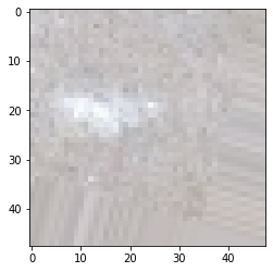
Let’s create functions to visualize images. For example to fetch an image through a given path. Just to check the size.

def get_image(path):
    img = cv2.imread(path)
    print(img.shape)
    plt.imshow(img)

Output:

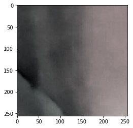
Image Data Generator

It generates batches of tensor image data with real-time data augmentation. There several parameters to pass in according to your need. Please check the documentation presented here.

Now, we will build our Image Data Generator which will be used to generate train and valid tests directly from the main directory by using Flow From Directory. We will also apply some image augmentation to our generator.

Rotation range of 20 degrees — rotates images randomly, set Horizontal and Vertical flip to be True, shifts in width and height, and the fill mode to be nearest. After initializing the generator, we will set the target size of each image to be 48×48(WxH).

Each image is required in color so we will set the color mode to be ‘RGB’. Batch size is the number of extractions from each subfolder. We will fit this generator for both sets i.e. train and valid.

traingen = datapreprocessing(train_dir,20)
validgen = datapreprocessing(test_dir,20)

Output:

Found 2249 images belonging to 4 classes.
Found 688 images belonging to 4 classes.

Let’s create a dictionary that contains labels for each class and keys for them. Later it will be used to fetch class names.

labelnames = traingen.class_indices
labelnames

Now, we will build a data frame that contains an absolute path to each image and its label.

#Create Train Dataframe as repository of paths and labels.
valid = getdata(test_dir)

Visualizing Images

Let’s create a function to visualize images. For example to fetch n number of images of good marble from the data frame.

This will be used later to visualize if the predictions are correct or not.

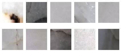
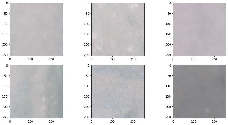
To visualize images from the generator, we will create another function.

visualize_gen(traingen)

Images look like this:

#Get the shape of images
input_shape = traingen.image_shape
input_shape

Model Architecture

The model will contain:

1. Two Conv2d layers
2. Two Dense Layers
3. Two MaxPoolinig and Dropout Layers

Conv2d layers will extract features from the images in pieces, Dense layer will tune up the weights for them. MaxPooling2D layer will reduce the dimensionality for easier computation and Dropout layers will avoid the overfitting of the model.

The model summary is given below:

Model: "sequential"
_________________________________________________________________
Layer (type)                 Output Shape              Param #   
=================================================================
layer1 (Conv2D)              (None, 48, 48, 8)         224       
_________________________________________________________________
max_pooling2d (MaxPooling2D) (None, 24, 24, 8)         0         
_________________________________________________________________
dropout (Dropout)            (None, 24, 24, 8)         0         
_________________________________________________________________
layer2 (Conv2D)              (None, 24, 24, 8)         584       
_________________________________________________________________
max_pooling2d_1 (MaxPooling2 (None, 12, 12, 8)         0         
_________________________________________________________________
flatten (Flatten)            (None, 1152)              0         
_________________________________________________________________
layer5 (Dense)               (None, 128)               147584    
_________________________________________________________________
dropout_1 (Dropout)          (None, 128)               0         
_________________________________________________________________
output (Dense)               (None, 4)                 516       
=================================================================
Total params: 148,908
Trainable params: 148,908
Non-trainable params: 0

Use the below code for building architecture.

model01 = imageclf2(input_shape)

Compile and Evaluate

To compile the model, we will use :

loss = categorical_crossentropy
optimizer = Adam
metrics = accuracy
callback = Earlystopping

Categorical cross-entropy as loss function because the task is multi-class classification. We will also use EarlyStopping callback to call the function back if it doesn’t improve after some epochs. We will do this by passing patience as a parameter to the callback.

Here’s the full code

Compile and evaluate the model on the validation dataset.

model_com01 = compiler2(model01,traingen,validgen,100)

Output:

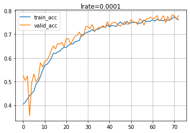
Restoring model weights from the end of the best epoch.
113/113 [==============================] - 5s 42ms/step - loss: 0.6710 - accuracy: 0.7617 - val_loss: 0.6584 - val_accuracy: 0.7791

Get Prediction and visualize the output.

Let’s try to predict any image available in the validation data set.

Pass in n any number between 0–19 because there are 20 images from each folder since we specified 20 as batch size during Image Generator initialization.

get_predictions(11)

Output:

array([2])

Let’s check if other good images are like this or not.

#Visualise Predictions
get_n_images(6,valid,"good")

The model has predicted that there is no deformation which is true.

Save the model!

# save the model to disk
model = model_com01[0]
model.save(\'saved_models/MarbleModel.tf\')

Thank you! for reading my story. Don’t forget to try different hyperparameters and see if the score can be improved.

Notebook Link: Here

Credit: Rishi Rajak

Also Read: Neural Style Transfer