Mushrooms!! Creamy Mushroom Bruschetta, Mushroom Risotto, Mushroom pizza, Mushrooms in a burger, and what not! Just by hearing the names of these dishes, people be drooling! Their flavor is one reason that takes the dish to the next level!

But have you ever wondered if the mushroom you eat is healthy for you? From over 14,000 species of mushrooms in the world, how will you classify the mushroom as edible or poisonous? Poisonous mushrooms can be hard to identify in the wild!

Introduction

In this project, we will examine the data and build a deep neural network model that will detect if the mushroom is edible or poisonous by its specifications like cap shape, cap color, gill color, etc. using different classifiers.

Dataset

The dataset used in this project is mushrooms.csv that contains 8124 instances of mushrooms with 23 features like cap-shape, cap-surface, cap-color, bruises, odor, etc.

We’ll use the specifications like cap shape, cap color, gill color, etc. to classify the mushrooms into edible and poisonous.

Let’s begin !!

Importing the necessary libraries

Let’s import the necessary libraries to get started with this task:

Reading the CSV file of the dataset

Pandas read_csv() function imports a CSV file (in our case, ‘mushrooms.csv’) to DataFrame format.

Examining the Data

After importing the data, to learn more about the dataset, we’ll use .head() .info() and .describe() methods.

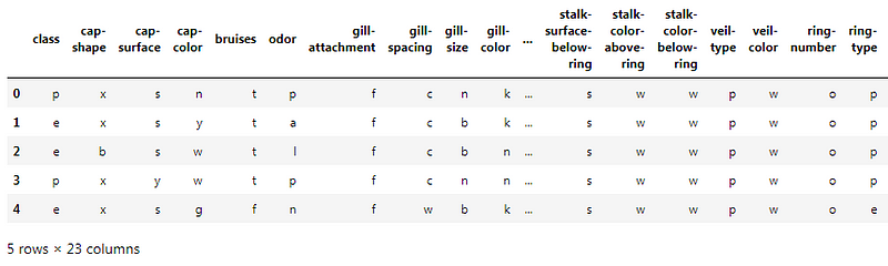
The .head() method will give you the first 5 rows of the dataset. Here is the output:

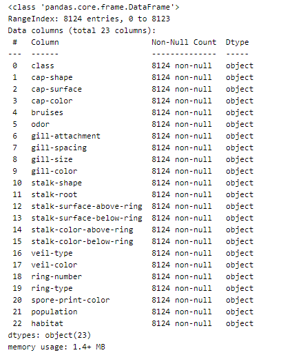
The .info() method will give you a concise summary of the DataFrame. This method will print the information about the DataFrame including the index dtype and column dtypes, non-null values, and memory usage. Here is the output:

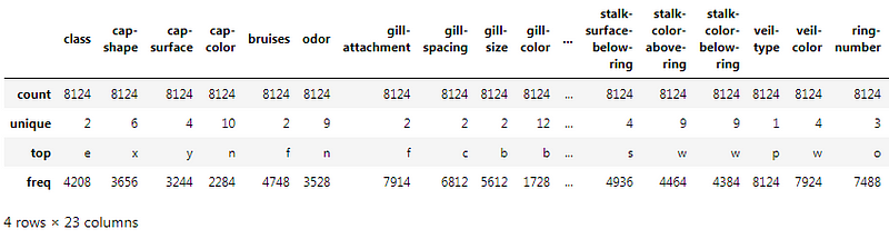
The .describe() method will give you the statistics of the columns.

• count shows the number of responses.
• unique shows the number of unique categorical values.
• top shows the highest-occurring categorical value.
• freq shows the frequency/count of the highest-occurring categorical value.

Here is the output:

The shape of the dataset

Dataset shape: (8124, 23)

This shows that our dataset contains 8124 rows i.e. instances of mushrooms and 23 columns i.e. the specifications like cap-shape, cap-surface, cap-color, bruises, odor, gill-size, etc.

Unique occurrences of ‘class’ column

The .unique() method will give you the unique occurrences in the ‘class’ column of the dataset. Here is the output:

array([\'p\', \'e\'], dtype=object)

As we can see, there are two unique values in the ‘class’ column of the dataset namely:

‘p’ -> poisonous and ‘e’ -> edible

Count of the unique occurrences of ‘class’ column

The .value_counts() method will give you the count of the unique occurrences. Here is the output:

e    4208
p    3916
Name: class, dtype: int64

As we can see, there are 4208 occurrences of edible mushrooms and 3916 occurrences of poisonous mushrooms in the dataset.

Now let’s visualize the count of edible and poisonous mushrooms using Seaborn :

Here, “count.index” represents the unique values i.e. ‘e’ and ‘p’, and “count.values” represents the count of those unique values i.e. 4208 and 3916 respectively. Here is the output of the bar graph:

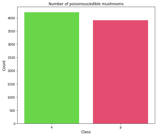
From the bar plot, we see that the dataset is balanced.

Data Manipulation

The data is categorical so we’ll one hot encoding to make the categorical data to numerical data.

Data Preparation

We will be using 80% of our dataset for training purposes and 20% for testing. It is not possible for us to manually split our dataset also we need to split the dataset in a random manner.

To help us with this task, we will be using a SciKit library named train_test_split. We will be using 80% of our dataset for training purposes and 20% for testing.

(1625, 117)

Now, let’s go ahead and build our Deep Learning model

A Sequential() the function is the easiest way to build a model in Keras. It allows you to build a model layer by layer. Each layer has weights that correspond to the layer the follows it. We use the add() function to add layers to our model.

Fully connected layers are defined using the Dense class. We can specify the number of neurons or nodes in the layer as the first argument, and specify the activation function using the activation argument.

We will use the rectified linear unit activation function referred to as ReLU on the first two layers and the Softmax function in the output layer.

ReLU is the most commonly used activation function in deep learning models. The function returns 0 if it receives any negative input, but for any positive value x it returns that value back. So it can be written as f(x)=max(0,x)

We will also use Dropout technique. Dropout is a technique where randomly selected neurons are ignored during training. They are “dropped out” randomly. This means that their contribution to the activation of downstream neurons is temporally removed on the forward pass and any weight updates are not applied to the neuron on the backward pass.

The softmax function is used as the activation function in the output layer of neural network models that predict a multinomial probability distribution. That is, softmax is used as the activation function for multi-class classification problems where class membership is required on more than two class labels.

Let’s build it :

Compiling the model

Now that the model is defined, we can compile it.

Compiling the model uses the efficient numerical libraries under the covers (the so-called backend) such as Theano or TensorFlow. The backend automatically chooses the best way to represent the network for training and making predictions to run on your hardware, such as CPU or GPU or even distributed.

We must specify the loss function to use to evaluate a set of weights, the optimizer is used to search through different weights for the network and any optional metrics we would like to collect and report during training.

In this case, we will use cross entropy as the loss argument. This loss is for a binary classification problems and is defined in Keras as “binary_crossentropy“. We will define the optimizer as the efficient stochastic gradient descent algorithm “sgd“.

Finally, because it is a classification problem, we will collect and report the classification accuracy, defined via the metrics argument.

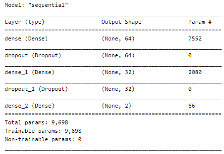
Model Summary

Let’s see our model’s summary :

Now, let’s fit the model :

We have defined our model and compiled it ready for efficient computation.

...
Epoch 10/15
204/204 [==============================] - 0s 2ms/step - loss: 0.0548 - accuracy: 0.9835 - val_loss: 0.0163 - val_accuracy: 0.9963
Epoch 11/15
204/204 [==============================] - 0s 2ms/step - loss: 0.0526 - accuracy: 0.9849 - val_loss: 0.0140 - val_accuracy: 0.9988
Epoch 12/15
204/204 [==============================] - 0s 2ms/step - loss: 0.0417 - accuracy: 0.9888 - val_loss: 0.0116 - val_accuracy: 0.9994
Epoch 13/15
204/204 [==============================] - 0s 2ms/step - loss: 0.0402 - accuracy: 0.9905 - val_loss: 0.0100 - val_accuracy: 0.9994
Epoch 14/15
204/204 [==============================] - 0s 2ms/step - loss: 0.0370 - accuracy: 0.9908 - val_loss: 0.0083 - val_accuracy: 0.9994
Epoch 15/15
204/204 [==============================] - 0s 2ms/step - loss: 0.0304 - accuracy: 0.9928 - val_loss: 0.0069 - val_accuracy: 0.9994

Model Evaluation

The evaluate() function will return a list with two values. The first will be the loss of the model on the dataset and the second will be the accuracy of the model on the dataset.

51/51 [==============================] - 0s 951us/step - loss: 0.0069 - accuracy: 0.9994
Accuracy: 99.94
Loss: 0.69

Now, let’s visualize the model training:

Let’s define a function for plotting the graphs.

Plotting the curves using the function defined above :

A history object contains all information collected during training.

Graphs :

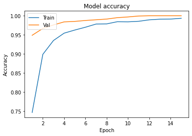
• In Model accuracy graph validation accuracy is always greater than train accuracy that means our model is not overfitting.
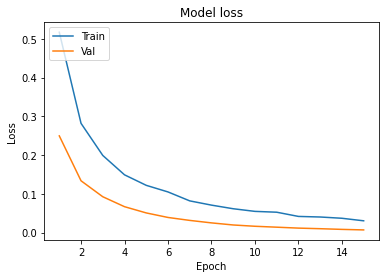
• In the Model loss graph validation loss is also very lower than training loss so unless and until validation loss goes above the training loss then we can keep training our model.

Making predictions on some values :

array([[1, 0],
       [1, 0],
       [0, 1],
       [0, 1],
       [1, 0],
       [1, 0],
       [0, 1],
       [0, 1],
       [1, 0],
       [0, 1]])

We have successfully created our model to classify mushrooms as poisonous/edible using Deep Neural Network.

Implementation of the project on cainvas here.

Credit : Jeet Chawla

fake chopard watches