Like every other plant, apple leaves are susceptible to many diseases. On a large scale, these diseases are harmful to the plants and an early diagnosis can help in early prevention ensuring plant quality.

Today, we aim to develop a neural network model which helps in this diagnosis by determining the apple leaf disease simply by “looking at it”.

With the help of this model, our objective is to classify the apple leaf disease into one of three categories, that are:
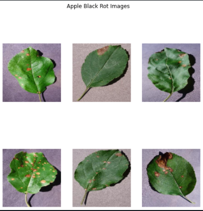
1. Apple Black Rot
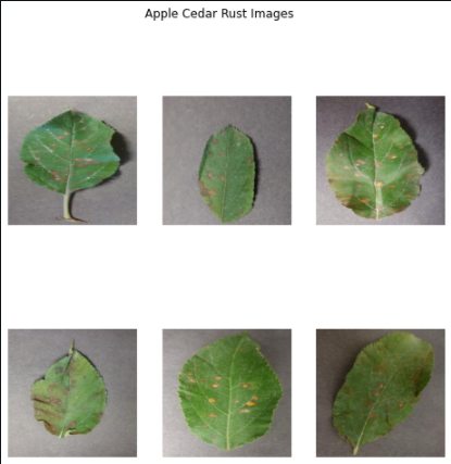
2. Apple Cedar Rust
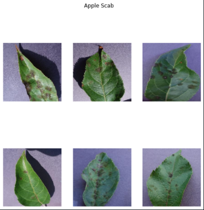
3. Apple Scab

For apple scab, leaf spots are round, olive-green in colour, and up to 0.5-inch across. These spots are velvet-like with fringed borders. Black rot is often recognized with symptoms such as purple spots on upper leaf surfaces.

As the spots age, the centers dry out and turn yellow to brown. Cedar rust is a fungal disease. Spores overwinter as a reddish-brown gall on young twigs. Sometimes, orange spots may develop on the fruit as well.

Firstly, we need a dataset on which we can train and prepare our model. The dataset can be accessed by the following link. Now that we have our dataset. The next thing we need is access to a platform that lets us train our DNN model. In order to do so, we can use the AITS Cainvas Platform. This gives us access to highly efficient GPUs and we can prepare our jupyter notebooks easily.

After importing all the libraries, we will create a ‘train_path’ variable that will access the directory containing the image files.

Since our data is not separated into training and validation images, we can either create new directories and split the data into training and validation folders or we can make do with this directory and create a validation split while pre-processing the data. We choose to proceed with the latter since it is more convenient.

Let us proceed with displaying some images in our notebook just to visualize the data we’re dealing with. We’ll display 6 images from each directory (each disease type) in different cells of our jupyter notebook.

Now that we know what kind of data we’re dealing with. Let us start with pre-processing our data. Since our images are less in number, we define training and validation image data generators to expand our dataset of training and validation images.

This is done by artificially generating new images by processing the existing images. By random flipping, rotating, scaling, and performing similar operations, we can create new images.

This creation is done with the help of ImageDataGenerator() function from the keras library. This pre-processing function is extremely helpful in dealing with image data. Next, we load our training and validation data through these image data generators and set an image input size of 64*64.

Since we do not have separate directories for training and validation data, we have added a validation split of 20% in the train image generator. This is done with the help of validation_split feature of Image Data Generator.

After defining the generators, we need to load our images to these functions and prepare them for further processing in the model.

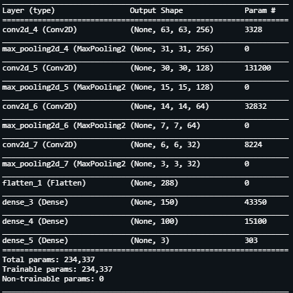
Now that we have our images which have been pre-processed and are ready to be read by our Neural Network Model, we define the architecture for it. We define a Sequential model with the following layers having about 235k trainable parameters.

For our model, every 2-dimensional convolution layer having a filter size of 2*2 is followed by a Max Pooling 2 Dimensional layer which has a similar filter size.

Now, we begin training our model. In the beginning, we defined a batch size of 20 for the images. We use this parameter for defining steps per epoch and validation steps.

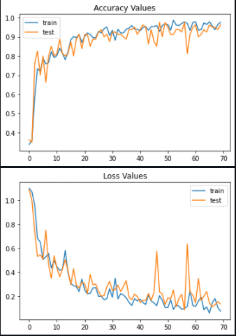
Training for 70 epochs ( or 70 iterations ) and with a learning rate of 0.001, we achieve a maximum training accuracy of about 98% and a maximum validation accuracy of about 97%. These values seem very promising. Next, let us visualize the training process of the model by monitoring the accuracy and loss values with respect to the number of epochs.

Using the model.evaluate() function, we evaluate the accuracy of our model solely on validation images. This metric confirms our earlier hypothesis and gives a validation accuracy of over 95%.
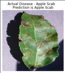
Lastly, we will predict on a random image from the apple scab directory.

When we select any random image using random.choice() and predict the disease, we observe that our model successfully predicts the right disease and thus ensures that our model is a success.

Using our Embedded ML knowledge, we have successfully developed a model which can predict the disease on apple leaves with great accuracy and thus, helping in an early diagnosis and an early precaution might help in curing the disease and improving crop yield.

If you want to access the entire notebook, follow this link.

Best of luck with your Machine Learning careers.
Cheers!

Notebook Link: Click Here

Credits: Kkharbanda

fakewatches.is