Computer Vision for Convenient Inventory Management

Retail especially daily needs and grocery stores have been traditional industries since quite a while now. With growing competition in terms of different competitors and increasing technological demands companies need to stay on their toes and up-to-date with innovations or risk staying behind.
This is where deep learning methods such as Computer Vision can come in and significantly change the experience for customers and businesses alike.
In this blog I will make a deep learning based classification tool which can classify grocery items into different categories for easier management. This use case can have a multitude of implementations in various tools and large scale projects. I hope you find this blog insightful and fun.
Applications of Deep Learning in Retail
- OCR for automated checkout.
- Realtime recommendation systems.
- Inventory management using computer vision.
- Make whole experience more friction-less.
Data and References
I have used Freiburg Groceries Dataset for this project. The paper and dataset can be found here.
Pre-requisites used
- Numpy
- Pandas
- Scikit-image
- Matplotlib
- Scikit-learn
- Keras
- Cainvas notebook
Here’s how it works
- Our input is a training dataset that consists of N images, each labeled with one of 5 different classes.
- Then, we use this training set to train a classifier to learn what every one of the classes looks like.
- In the end, we evaluate the quality of the classifier by asking it to predict labels for a new set of images that it has never seen before. We will then compare the true labels of these images to the ones predicted by the classifier.
Code
Let’s get started with the code. It can be found on the Cainvas platform over here.
Loading all the dependencies.
https://gist.github.com/242c277337e4c0e32d78459a1732a328
This is a function to plot loss and accuracy which we will get after training the model.
https://gist.github.com/b3f06260497ae1b756afca84fe4b7037
Defining a function to return the label of a particular image and load the dataset by appending the labels to the training data for each class.
https://gist.github.com/b3f2f956beb0e22a40a4693e1057b5a7
Data Augmentation
The images present in the ship class are augmented and then stored in the dataset, so that there is an equal representation of the classes.
The current ratio of classes is 1:3, meaning that for every image present in the ship class there are 3 images present in the no-ship class. This will be countered by producing 2 augmented images per original image of the ship class. This will make the dataset balanced.
Then the labels NumPy array is one hot encoded using to_categorical from Keras. This removes any unnecessary bias in the dataset, by keeping the class at equal footing, with respect to labels.
https://gist.github.com/4a18ad907c8681520e5f1cc937eb4e02
https://gist.github.com/40be672f3ead95919ec8d6d2a0dfc0cd
Splitting the data
Instead of using train_test_split the images and labels arrays are randomly shuffled using the same seed value set at 42. This allows the images and their corresponding labels to remain linked even after shuffling.
This method allows the user to make all 3 datasets. The training and validation dataset is used for training the model while the testing dataset is used for testing the model on unseen data. Unseen data is used for simulating real-world prediction, as the model has not seen this data before. It allows the developers to see how robust the model is.
The data has been split into –
- 70% — Training
- 20% — Validation
- 10% — Testing
https://gist.github.com/2eee5638f74800b5fd039f3bc33915c9
Model Architecture
Our model structure consists of four Conv2D layers including the input layer with a 2×2 MaxPool2D pooling layer each followed by a dense layer of 64 neurons and one dense layer of 64 neurons each with a ReLU activation function and the last layer with 5 neurons and the softmax activation function for making our class predictions.
https://gist.github.com/a78fcdfebad5da2a8ee71210cf8fcc0e
Model: "sequential"
_________________________________________________________________
Layer (type)                 Output Shape              Param #
=================================================================
zero_padding2d (ZeroPadding2 (None, 106, 106, 3)       0
_________________________________________________________________
conv2d (Conv2D)              (None, 104, 104, 32)      896
_________________________________________________________________
batch_normalization (BatchNo (None, 104, 104, 32)      128
_________________________________________________________________
max_pooling2d (MaxPooling2D) (None, 52, 52, 32)        0
_________________________________________________________________
dropout (Dropout)            (None, 52, 52, 32)        0
_________________________________________________________________
conv2d_1 (Conv2D)            (None, 50, 50, 32)        9248
_________________________________________________________________
max_pooling2d_1 (MaxPooling2 (None, 25, 25, 32)        0
_________________________________________________________________
dropout_1 (Dropout)          (None, 25, 25, 32)        0
_________________________________________________________________
conv2d_2 (Conv2D)            (None, 23, 23, 32)        9248
_________________________________________________________________
max_pooling2d_2 (MaxPooling2 (None, 11, 11, 32)        0
_________________________________________________________________
dropout_2 (Dropout)          (None, 11, 11, 32)        0
_________________________________________________________________
conv2d_3 (Conv2D)            (None, 9, 9, 32)          9248
_________________________________________________________________
max_pooling2d_3 (MaxPooling2 (None, 4, 4, 32)          0
_________________________________________________________________
dropout_3 (Dropout)          (None, 4, 4, 32)          0
_________________________________________________________________
conv2d_4 (Conv2D)            (None, 2, 2, 32)          9248
_________________________________________________________________
max_pooling2d_4 (MaxPooling2 (None, 1, 1, 32)          0
_________________________________________________________________
dropout_4 (Dropout)          (None, 1, 1, 32)          0
_________________________________________________________________
flatten (Flatten)            (None, 32)                0
_________________________________________________________________
dense (Dense)                (None, 64)                2112
_________________________________________________________________
dropout_5 (Dropout)          (None, 64)                0
_________________________________________________________________
dense_1 (Dense)              (None, 5)                 325
=================================================================
Total params: 40,453
Trainable params: 40,389
Non-trainable params: 64
_________________________________________________________________
I defined checkpoints specifying when to save the model and implemented early stopping to make the training process more efficient.
https://gist.github.com/8cd1fd71c01bf582c255c880a6b452ed
I have used Adam as the optimizer as it was giving much better results. I have used binary cross-entropy as the loss function for our model. I trained the model for 200 iterations.
However, you’re free to use a number of different parameters to your liking as long as the accuracy of the predictions doesn’t suffer.
https://gist.github.com/924742261d32260ef329ad3065d13f4d
The model was saved and the results were plotted using the earlier defined function.
https://gist.github.com/3af7e66a9fce537b1afbf7909b936ae3
Results
Loss/Accuracy vs Epoch
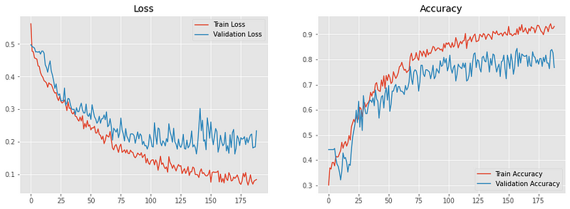
The model is able to reach a validation accuracy of 84% which is decent.
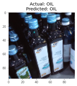
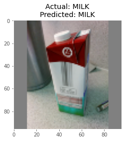
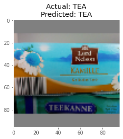
Predictions
Here are some of the predictions made by the model on the test data:
Future Scope
- Dataset used should be specific to a country/region for getting predictions more accurate to that specific region’s products.
- Larger dataset to build a more robust model.
Conclusion
In this article, I’ve demonstrated how a ConvNet built from scratch can be used in inventory management by detecting grocery items using deep learning.
This simple use-case can be used as a module in more complex frameworks for achieving object detection where the products can be detected and marked out from images of the product shelves.
Notebook Link : Here
Credit: Ved Prakash Dubey