Train a model to identify if the sonar wave bounced off a rock or mine in the ocean.

Sonar (sound navigation and ranging) is a technique based on the principle of reflection of ultrasonic sound waves. These waves propagate through water and reflect on hitting the ocean bed or any object obstructing its path.
Sonar has been widely used in submarine navigation, communication with or detection of objects on or under the water surface (like other vessels), hazard identification, etc.
There are two types of sonar technology used — passive (listening to the sound emitted by vessels in the ocean) and active (emitting pulses and listening for their echoes).
It is important to note that research shows the use of active sonar can cause mass strandings of marine animals.
Implementation of the idea on cAInvas — here!
The dataset
This dataset was used in Gorman, R. P., and Sejnowski, T. J. (1988). “Analysis of Hidden Units in a Layered Network Trained to Classify Sonar Targets” in Neural Networks, Vol. 1, pp. 75–89.
The CSV files contain data regarding sonar signals bounced off a metal cylinder (mines — M) and a roughly cylindrical rock (rock — R) at various angles and under various conditions.
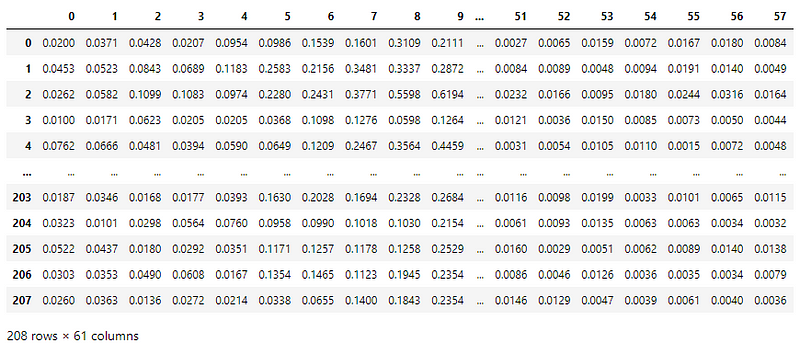
There are 60 attributes and one categorical column in the dataset.
Looking into the spread of categorical values in the dataset.
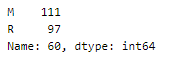
It is a fairly balanced dataset.
Preprocessing
Categorical features
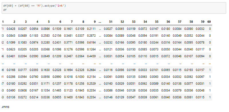
The category column has R and M to denote the classes. We have to convert them into numeric values.
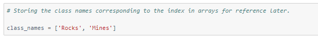
Now that we have re-labeled the classes, we will define class names accordingly for later use.
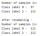
Balancing the dataset
Even though there is only a difference of only 14 samples, in comparison to the total number of data samples available, this difference is significant and needs to be balanced.
In order to balance the dataset, there are two options,
- upsampling — resample the values to make their count equal to the class label with the higher count (here, 111).
- downsampling — pick n samples from each class label where n = number of samples in class with least count (here, 97)
Here, we will be upsampling. First, we divide the whole dataset into 2, one for each label. The sample() function of the data frame is used to resample and obtain 9200 samples. The append() function of the data frame is used to combine the rows in both the datasets.
Defining the input and output columns
We define the columns of the data frame to be used as input and output for the model.
There are 60 input columns and 1 output column.
Train-val split
Splitting the dataset into training and validation sets using a 90–10 split ratio. The datasets are then split into respective X and y arrays for further processing.
The training set has 199 samples and the validation set has 23 samples.
Here is a peek into the distribution of samples in the training and validation sets.
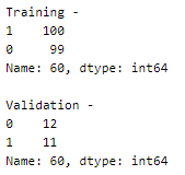
Seems balanced!
Standardization
The range of values for the attributes are almost of the same range, but the little difference has caused a shift of the means.
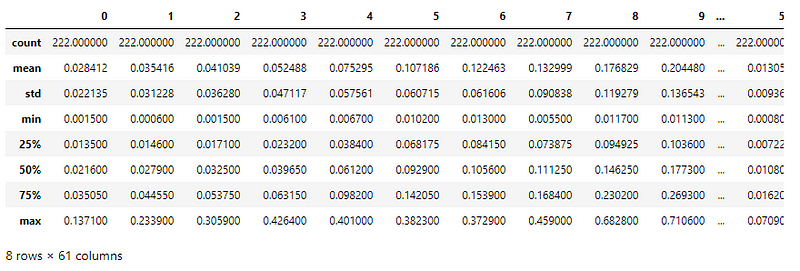
Using the StandardScaler() function of the sklearn.preprocessing module to scale the values to have a mean = 0 and variance = 1.
The StandardScaler instance is fit on the training input data and used to transform the train, validation, and test sets.
The model
The model is a simple one with 4 Dense layers where the 3 initial layers use the ReLU activation function and the last one uses the Sigmoid activation function.
The model is compiled using the Binary cross-entropy loss function because the final layer of the model performs a two-class classification using the sigmoid activation function. The Adam optimizer is used and the accuracy of the model is tracked over epochs.
The EarlyStopping callback function of the keras.callbacks module monitors the validation loss and stops the training if it doesn’t for 3 epochs continuously. The restore_best_weights parameter ensures that the model with the least validation loss is restored to the model variable.
The model is trained first with a learning rate of 0.01 which is then reduced to 0.001.
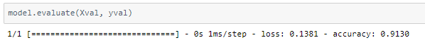
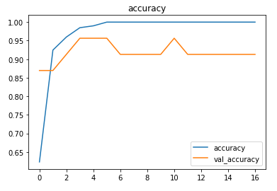
The model achieved around 91% accuracy on the validation set.
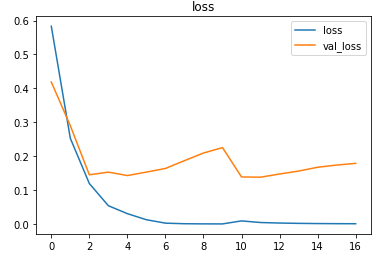
The metrics
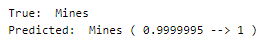
Predictions
Let’s perform predictions on random test data samples —
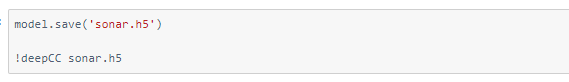
deepC
deepC library, compiler, and inference framework are designed to enable and perform deep learning neural networks by focussing on features of small form-factor devices like micro-controllers, eFPGAs, CPUs, and other embedded devices like raspberry-pi, odroid, Arduino, SparkFun Edge, RISC-V, mobile phones, x86 and arm laptops among others.
Compiling the model using deepC —
Head over to the cAInvas platform (link to notebook given earlier) and check out the predictions by the .exe file!
Credits: Ayisha D
Also Read: Mineral Classification