
Stroke Detection using Neural Networks – Strokes mostly caused by loss or reduction of oxygen supply to the brain. This loss of supply is brought about by loss of blood or damage to the blood vessels.
In this article, we attempt to use our Embedded Machine Learning and Deep Learning skills to predict the onset of a stroke based upon the lifestyle of a person. We consider several relevant factors such as age, Body Mass Index (BMI), Marital Status, Smoking Status, and many more. In order to access the dataset, you can follow this link .
Right, now that we have the data, we need a platform where we can perform our data visualization, pre-processing and training of our neural network classifier. In order to do so, we can use the AITS Cainvas Platform. This gives us access to highly efficient GPUs and we can prepare our jupyter notebooks easily.
We’ll start with uploading the data and access it using the pandas library. Pandas is a library which provides easy-to-use data structures for storing information, performing visualization tasks and pre-process the data with the help of other libraries.
We drop the “ID” column since it has absolutely no relevance in determining the occurrence of a stroke. Next step is to deal with the “NULL” values in the data. We observe that only bmi column has NULL values so we tackle the problem by filling it with the mean bmi value. In order to learn more techniques for deal with missing data, you can follow this link.
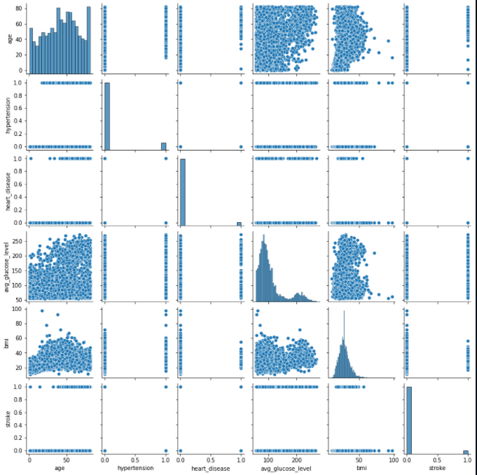
After the missing data has been dealt with, the next step is to perform data visualization tasks in order to understand the complexity of the data.
We deal with several plots in order to understand the relationship of the data using the seaborn library and matplotlib. Starting off with a countplot to check the distribution of our data. We observe that our data is highly unbalanced with one class being over-represented than the other.
Further, we study the effect of smoking and age on stroke occurrence. By analyzing the graph, we understand that individuals who are aged and tend to smoke have a higher chance of suffering a stroke when compared to young non-smokers.
Next, we attempt to understand the affect of marital status of a person on stroke occurrence.
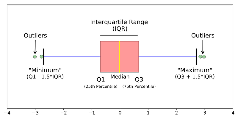
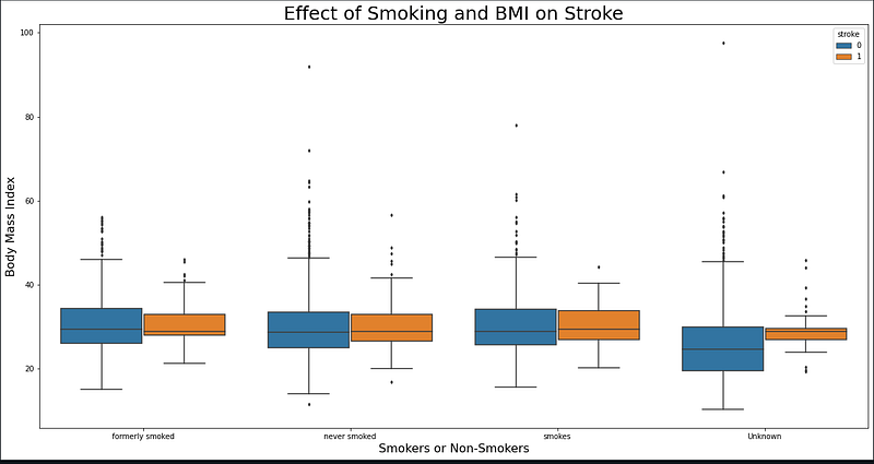
This is followed by a boxplot which helps us understand the effect the Body Mass Index (BMI) and Smoking Status on strokes.
A boxplot is a very informative way of potraying the distribution of data along the following measures:
1. Outliers of the data
2. Minimum value of the data
3. First Quartile (Q1–25th Percentile)
4. Median value
5. Third Quartile (Q3–75th Percentile)
6. Maximum value of the data
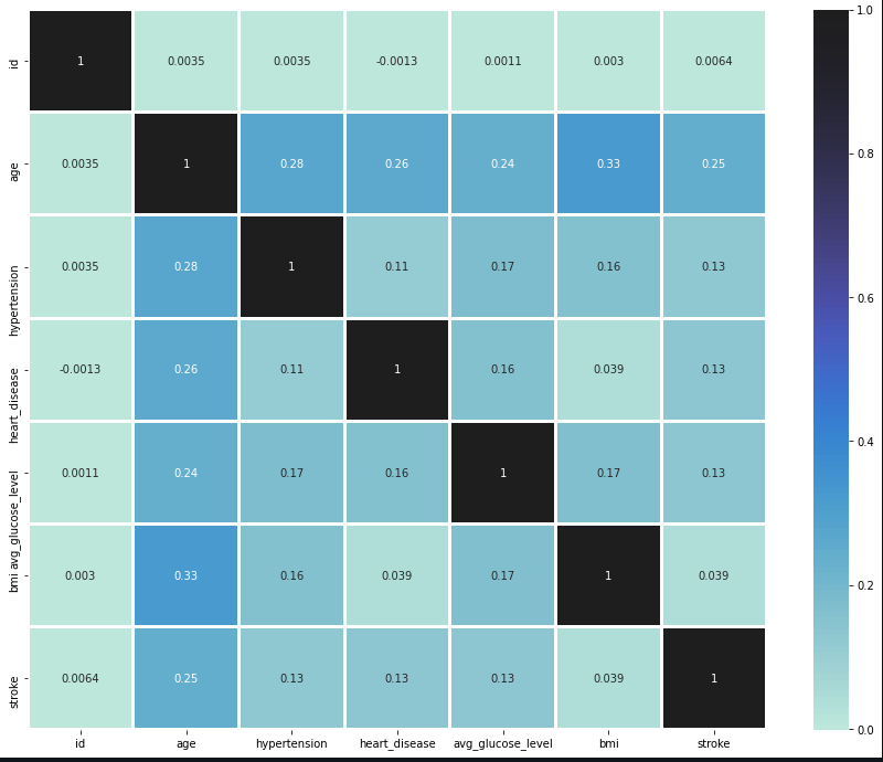
Finally, in an attempt to understand the relation between all the columns, we plot a heatmap annotated with the correlation values.
After data visualization, we need to start pre-processing our data to train a Neural Network model. We observe that our data contains information in the form of text-classes. In order to make our model understand the data, we need to convert this data into numerical format. To accomplish this task, we use LabelEncoder on all the relevant columns.
Next step is to split the data into training and test parts with a split of 40% for testing and 60% for training. After splitting the data, we standardize it by removing the mean and scaling to unit variance using StandardScalar() function on the training data.
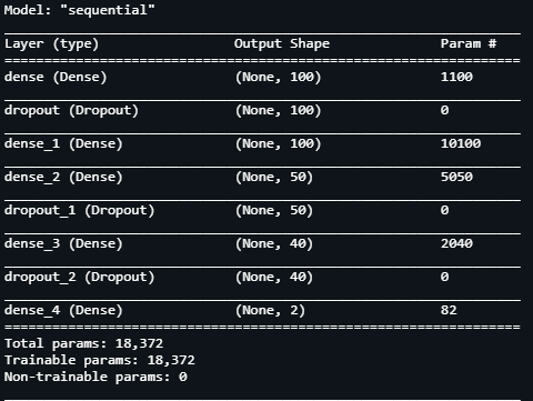
After the data is ready, we need to prepare the model. Starting with the architecture, our Neural Network model consists of 5 Dense layers and 3 Dropout layers having a drop value of 30% each. We view the summary of the model and conclude that there are over 18k parameters for our model.
After compiling the model using Adam optimizer and a learning rate of 0.1, we set the loss function to categorical cross entropy, we begin our training.
In order to train our model and prevent any over-fitting, we set up an EarlyStopping check which monitors our validation loss. We begin training our model and for 100 epochs which stops after about 7–8 epochs due to our check function on validation loss.
We achieve great validation accuracy exceeding 95%. To plot the training curves on our model to observe the accuracy and loss values with each epoch, we use the following function.
Our final check is to make some predictions on the testing data which we evaluate using a confusion matrix. After making predictions, we can plot our confusion matrix using the following code:
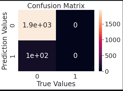
Our model is a success based on the data. We have finally completed this project and can conclude the advantages of Machine Learning and Deep Learning industry are immeasurable. We, as machine learners can use our skill and knowledge effectively and can give back to the society by making huge progress in fields such as healthcare.
If you’d like to learn more and access the full notebook, you can do it by following this link.
Best of luck for your Machine Learning career! Cheers!
Notebook Link: Here
Credit: Kkharbanda
Also Read: Lower Back Pain Symptoms Detection using NN