Using convolutional neural networks to classify heartbeat sounds into five categories.

Arrhythmia refers to an irregularity in the rate or rhythm of the heartbeat. This includes beating too fast or too slow or with an irregular rhythm.
Deep learning models have proven useful and very efficient in the medical field to process scans, x-rays, and other medical data to output useful information.
In this article, we use deep learning to classify heartbeats into five categories.
A link to the implementation on cAInvas — here.
Dataset
Data source: Physionet’s MIT-BIH Arrhythmia Dataset
The signals in the dataset correspond to electrocardiogram (ECG) shapes of heartbeats for the normal case and the cases affected by different arrhythmias and myocardial infarction. These signals are preprocessed and segmented, with each segment corresponding to a heartbeat.
The dataset has 2 CSV files, one containing samples for training and the other for testing. The train.csv file has 87,554 samples.
Here is a peek into the train.csv file —
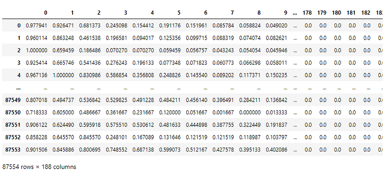
Each sample, in the train and test file, has 187 input features and one column that indicates the classification labels.
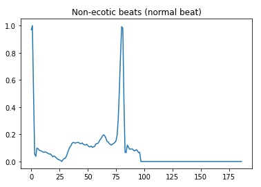
The heartbeats in the dataset fall into five categories as below —
- 0 — Non-ectopic beats (normal beat)
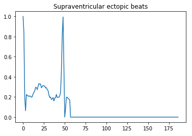
- 1 — Supraventricular ectopic beats
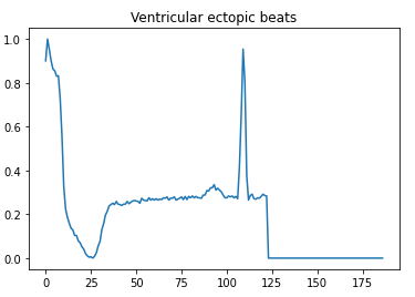
- 2 — Ventricular ectopic beats
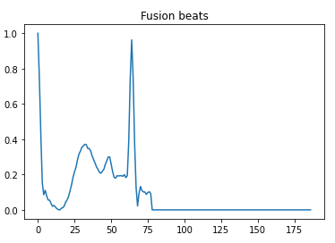
- 3 — Fusion beats
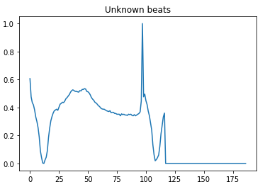
- 4 — Unknown beats
Let us see the spread of samples across the labels —
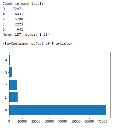
The dataset is very imbalanced.
There are two ways to balance this dataset —
- Limiting samples from the class with a higher count to match that with the lower count.
- Resampling samples from the class with a lower count in order to match the count of the class with a higher count.
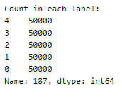
To do this, we will first separate the dataset into five, each containing samples belonging to a particular class.
Each dataset is then resampled to get 50000 samples in each.
The five datasets are then concatenated to get a balanced dataset with 250000 samples in total.
Here is a visual peek into the different class of heartbeats —
Preprocessing
Adding noise
Noise is added to the data to mimic the external random processes that can interfere in the data recording process. Additive white Gaussian noise (AWGN) is a widely used model for this.
It is additive because the generated noise is added to the existing noise in the system. White noise refers to a random signal having uniform intensity at different frequencies, thus having a constant power spectrum density. The noise is gaussian because it has a normal distribution across the time domain.
This function adds noise to the signal passed as a parameter. Feel free to play around with the standard deviation hyperparameter (here, 0.05) and visualize the signal with noise.
The first 187 columns are taken as the input signal in both the train and test datasets.
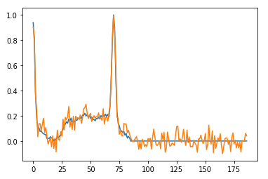
Here is a sample signal with added noise —
One hot encoding
The class labels of the dataset are integers (0–4). Since this is a classification problem, the class labels are one hot encoded using the keras.utils.to_categorical function.
Sample one hot encoding: Integer value 1 → [0, 1, 0, 0, 0]
The model
The model has three pairs of Convolution1D-MaxPool1D layers followed by a Flatten layer that reduces the values to 1D. This is then followed by 3 Dense layers, two of which have ReLU activation function while the last layer has 5 nodes, corresponding to the 5 output class labels, with a Softmax activation function.
The softmax activation function is used when the outputs given to train are one hot encoded as this function turns a vector of n values into a vector with n values that sum to 1, thus representing the probability of each class represented by the n values.
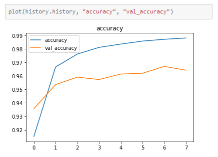
The model was able to achieve ~96% accuracy on the test dataset.
But, as we recall, only the training data was balanced. This means that the test dataset is still unbalanced and maybe the reason for the high accuracy value.
In the case of unbalanced datasets, the f1 score is a good measure of the model’s usability.
But before that let us plot the confusion matrix to see the performance of the model on various classes.
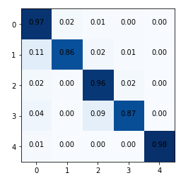
Looks like our model is performing well across all classes.
Let us now calculate the f1 score —
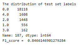
Given that the test set is also highly imbalanced, the decent f1-score indicates a reasonably well-performing model.
The metrics
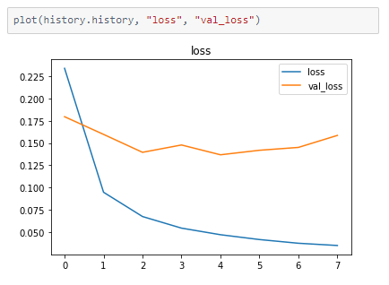
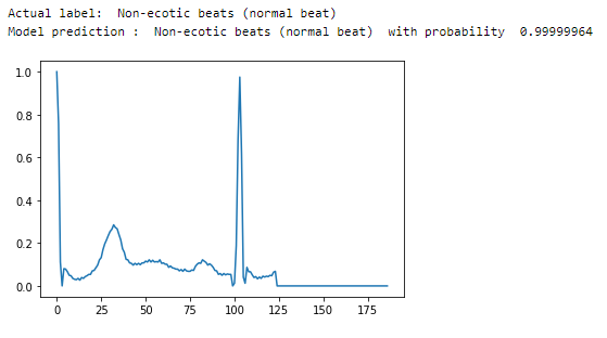
Prediction
Let’s randomly visualize some of the heartbeat signals while performing predictions using our model.
deepC
deepC library, compiler, and inference framework are designed to enable and perform deep learning neural networks by focussing on features of small form-factor devices like micro-controllers, eFPGAs, CPUs, and other embedded devices like raspberry-pi, odroid, Arduino, SparkFun Edge, RISC-V, mobile phones, x86 and arm laptops among others.
Compiling the model with deepC to get .exe file —
Head over to the cAInvas platform (link to notebook given earlier) and check out the predictions by the .exe file!
Credit: Ayisha D
Also Read: Neural Machine Translator