Breast cancer is the most commonly occurring cancer in women and the second most common cancer overall. There were over 2.3 million new cases in 2020, making it a significant health problem in the present day.

The key challenge in breast cancer detection is to classify tumors as malignant or benign. Malignant refers to cancer cells that can invade and kill nearby tissue and spread to other parts of your body. Unlike cancerous tumors (malignant), Benign does not spread to other parts of the body and is safe somehow. Deep neural network techniques can be used to improve the accuracy of early diagnosis significantly.

Deep Learning is a subfield of machine learning concerned with algorithms inspired by the structure and function of the brain called an artificial neural network.

A Convolutional Neural Network (ConvNet/CNN) is a Deep Learning algorithm that can take in an input image, assign importance (learnable weights and biases) to various aspects/objects in the image, and be able to differentiate one from the other. The pre-processing required in a ConvNet is much lower as compared to other classification algorithms.

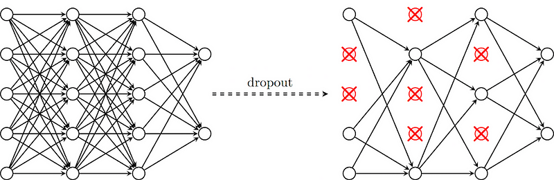
What is Dropout

Dropout is a technique where randomly selected neurons are ignored during training. They are “dropped out” randomly. This means that their contribution to the activation of downstream neurons is temporally removed on the forward pass and any weight updates are not applied to the neuron on the backward pass.

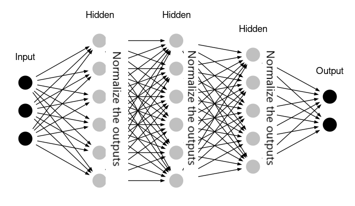
What is Batch Normalization

• It is a technique that is designed to automatically standardize the inputs to a layer in a deep learning neural network.
  e.g. We have four features having different units after applying batch normalization it comes in a similar unit.
• By Normalizing the output of neurons the activation function will only receive inputs close to zero.
• Batch normalization ensures a non-vanishing gradient.

Let’s begin !!

Importing the necessary libraries

Let’s import the necessary libraries to get started with this task:

About the dataset

For this problem statement, we will be using the famous Breast Cancer Wisconsin (Diagnostic) Data Set. Features are computed from a digitized image of a fine needle aspirate (FNA) of a breast mass. They describe the characteristics of the cell nuclei present in the image.

Also can be found on UCI Machine Learning Repository: https://archive.ics.uci.edu/ml/datasets/Breast+Cancer+Wisconsin+%28Diagnostic%29

Attribute Information:

1. Diagnosis (M = malignant, B = benign)
2. Ten real-valued features are computed for each cell nucleus:

a) radius (mean of distances from the center to points on the perimeter)
b) texture (standard deviation of gray-scale values)
c) perimeter
d) area
e) smoothness (local variation in radius lengths)
f) compactness (perimeter² / area — 1.0)
g) concavity (severity of concave portions of the contour)
h) concave points (number of concave portions of the contour)
i) symmetry
j) fractal dimension (“coastline approximation” — 1)

The mean, standard error, and “worst” or largest (mean of the three largest values) of these features were computed for each image, resulting in 30 features. For instance, field 3 is Mean Radius, field 13 is Radius SE, field 23 is Worst Radius.

All feature values are recoded with four significant digits.

Missing attribute values: none

Class distribution: 357 benign, 212 malignant

Loading of data and looking into some insights

The dataset is already present in the sklearn.datasets module. The breast cancer dataset is a classic and very easy binary classification dataset.

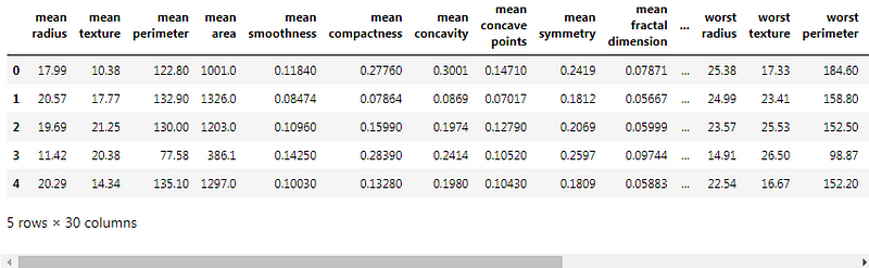
We will be using pandas DataFrame to present all our data. We will create a dataframe with our cancer data and target data. It would help us to store all the inputs and outputs in one dataframe.

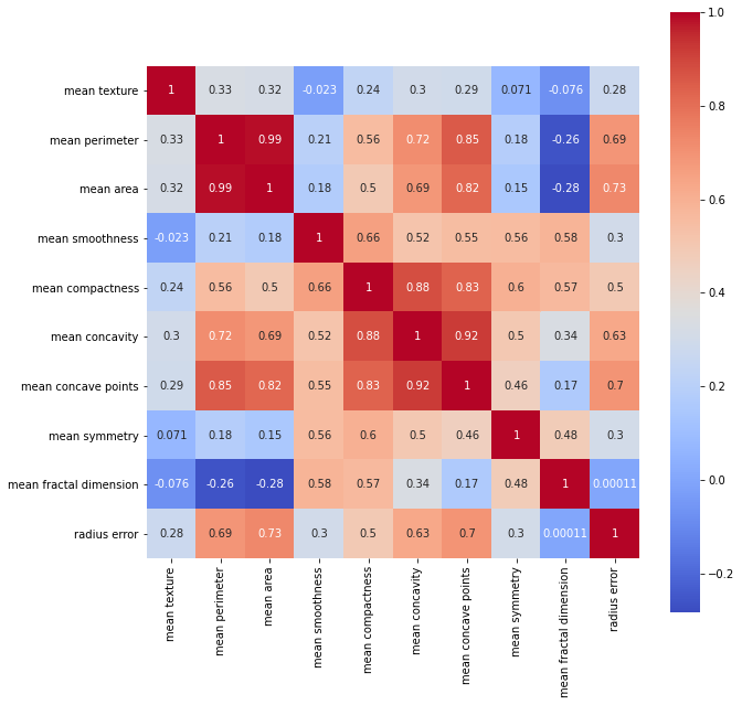
Let’s find the correlation between some columns :

Description of data :

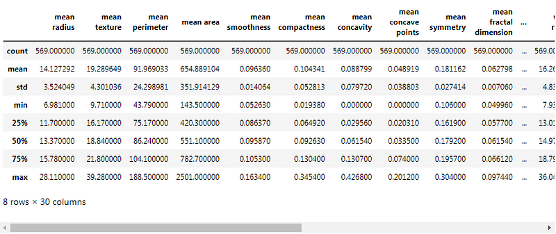
Data Splitting and Standardization

In this section, we will be splitting our dataset into training and testing parts. Also, we will be using standardization on this data.

(569, 30)

(569,)

array([\'malignant\', \'benign\'], dtype=\'<U9\')

We will be using 80% of our dataset for training purposes and 20% for testing. It is not possible for us to manually split our dataset also we need to split the dataset in a random manner. To help us with this task, we will be using a SciKit library named train_test_split. We will be using 80% of our dataset for training purposes and 20% for testing.

(455, 30)
(114, 30)

StandardScaler removes the mean and scales the data to unit variance :

Now, Let’s go ahead and build our CNN model

A Sequential() the function is the easiest way to build a model in Keras. It allows you to build a model layer by layer. Each layer has weights that correspond to the layer the follows it. We use the add() function to add layers to our model.

Conv1D() is a 1D Convolution Layer, this layer is very effective for deriving features from a fixed-length segment of the overall dataset, where it is not so important where the feature is located in the segment.

In the first Conv1D() layer, we are learning a total of 36 filters with the size of the convolutional window as 3. The input_shape specifies the shape of the input. It is a necessary parameter for the first layer in any neural network.

We will be using the ReLu activation function. The rectified linear activation function or ReLU for short is a piecewise linear function that will output the input directly if it is positive, otherwise, it will output zero.

The Rectified Linear Unit(ReLu) is the most commonly used activation function in deep learning models. The function returns 0 if it receives any negative input, but for any positive value x it returns that value back. So it can be written as f(x)=max(0,x)

To stop problem of shrinkage of data we use concept called Padding.

It has two types:

• valid
• same

Flattening is converting the data into a 1-dimensional array for inputting it to the next layer. We flatten the output of the convolutional layers to create a single long feature vector.

The Sigmoid function takes a value as input and outputs another value between 0 and 1. It is non-linear and easy to work with when constructing a neural network model. The good part about this function is that continuously differentiable over different values of z and has a fixed output range.

Let’s build it and visualize the summary :

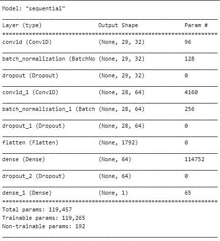
Compile defines the loss function, the optimizer, and the metrics. That’s all. It has nothing to do with the weights and you can compile a model as many times as you want without causing any problem to pretrained weights.

Now, let’s fit the model :

...
Epoch 46/50
15/15 [==============================] - 0s 3ms/step - loss: 0.1053 - accuracy: 0.9604 - val_loss: 0.1078 - val_accuracy: 0.9737
Epoch 47/50
15/15 [==============================] - 0s 3ms/step - loss: 0.1248 - accuracy: 0.9560 - val_loss: 0.1068 - val_accuracy: 0.9649
Epoch 48/50
15/15 [==============================] - 0s 3ms/step - loss: 0.1143 - accuracy: 0.9560 - val_loss: 0.1060 - val_accuracy: 0.9649
Epoch 49/50
15/15 [==============================] - 0s 3ms/step - loss: 0.1078 - accuracy: 0.9560 - val_loss: 0.1054 - val_accuracy: 0.9649
Epoch 50/50
15/15 [==============================] - 0s 3ms/step - loss: 0.0932 - accuracy: 0.9670 - val_loss: 0.1064 - val_accuracy: 0.9649

Now, let’s visualize the model training:

Plotting the curves using the function defined above :

A history object contains all information collected during training.

Graphs :

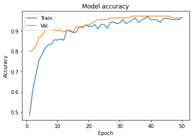
• In Model accuracy graph validation accuracy is always greater than train accuracy that means our model is not overfitting.
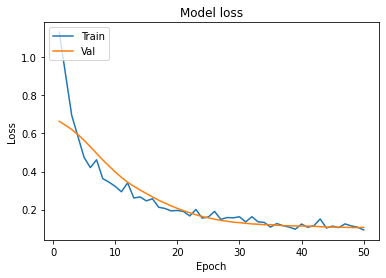
• In the Model accuracy graph validation loss is also very lower than training loss so unless and until validation loss goes above the training loss then we can keep training our model.

Making predictions on some values :

[[0]
 [0]
 [0]
 [1]
 [0]
 [1]
 [0]
 [1]
 [1]
 [0]]

We have successfully created our program to detect breast cancer using Deep Neural Network. We are able to classify cancer effectively with our CNN technique.

Implementation of the project on cainvas here.

Credit: Jeet Chawla