Detect epileptic seizures in patients using continuously monitored EEG data.
A sudden rush of electric activity in the brain is called a seizure. Seizures can either be generalized (affecting the whole brain) or focussed (affecting one part of the brain).
Epilepsy is a chronic neurological disorder causing involuntary, recurrent seizures. Some people stare blankly during a seizure while others may experience repeated twitching of their limbs. They last around 2 minutes in most cases and the patients take some time to return to normal.
An epileptic diagnosis requires at least two unprovoked seizures. A doctor uses various symptoms, electroencephalogram (EEG), computed tomography (CAT), Magnetic resonance imaging (MRI), and other tests to arrive at a diagnosis.
Deep learning can be used to detect and monitor seizures in patients and IoT provides ease of integration with the existing health system and patient wearability.
The implementation of the idea on cAInvas — here!
The dataset
Citation:
Andrzejak RG, Lehnertz K, Rieke C, Mormann F, David P, Elger CE (2001) Indications of nonlinear deterministic and finite dimensional structures in time series of brain electrical activity: Dependence on recording region and brain state, Phys. Rev. E, 64, 061907
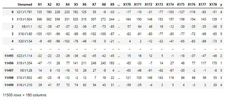
The CSV file consists of processed EEG recordings of patients at different points in time.
The original dataset has 5 different folders, each with 100 files, with each file representing a single subject/person. Each file is a recording of brain activity for 23.6 seconds. The corresponding time-series is sampled into 4097 data points.
This was then divided and shuffled into 23 chunks, each chunk containing 178 data points for 1 second, and each data point is the value of the EEG recording at a different point in time. Thus, we have 23 x 500 = 11500 pieces of information, each information contains 178 data points for 1 second.
The last column contains the categorical variable with the following values –
- 5 — Recording the EEG signal of the brain when the patient had their eyes open
- 4 — Recording the EEG signal when the patient had their eyes closed
- 3 — Recording the EEG activity from the healthy brain area
- 2 — Recording the EEG from the area where the tumor was located
- 1 — Recording of seizure activity
Here, only label 1 corresponds to seizure activity.
We will be training the model to identify patients with seizure activity against the rest of the classes.
Preprocessing
Re-labeling
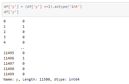
As we will be classifying samples into two categories, epileptic (label 1) and non-epileptic (labels 2, 3, 4, 5), we will change the labels in the data frame.
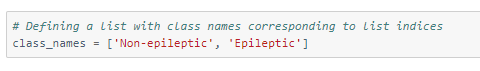
Now that we have re-labeled the classes, we will define class names accordingly for later use.
Let us look at the spread of values in different classes.
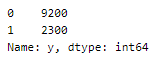
This was a balanced set with 5 labels that we have now re-labeled into an unbalanced set!
Resampling
In order to balance the dataset, there are two options,
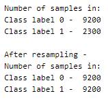
- upsampling — resample the values to make their count equal to the class label with the higher count (here, 9200).
- downsampling — pick n samples from each class label where n = number of samples in class with least count (here, 2300)
Here, we will be upsampling. First, we divide the whole dataset into 2, one for each label. The sample() function of the data frame is used to resample and obtain 9200 samples. The append() function of the data frame is used to combine the rows in both the datasets.
Defining the input and output columns
We define the columns of the data frame to be used as input and output for the model.
There are 178 input columns and 1 output column.
Train-val-test split
Splitting the dataset into training, validation, and test sets using an 80–10–10 split ratio. The datasets are then split into respective X and y arrays for further processing.
Standardization
All the features have a similar range of values. But they are skewed differently as their mean values indicate.
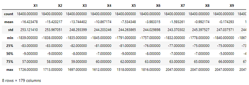
Using the StandardScaler() function of the sklearn.preprocessing module to scale the values to have a mean = 0 and variance = 1.
The StandardScaler instance is fit on the training input data and used to transform the train, validation, and test sets.
The model
The model is a simple one with 4 Dense layers where the 3 initial layers use the ReLU activation function and the last one uses the Sigmoid activation function.
The model is compiled using the Binary cross-entropy loss function because the final layer of the model has the sigmoid activation function. The Adam optimizer is used and the accuracy of the model is tracked over epochs.
The EarlyStopping callback function monitors the validation loss and stops the training if it doesn’t for 3 epochs continuously. The restore_best_weights parameter ensures that the model with the least validation loss is restored to the model variable.
The model is trained first with a learning rate of 0.01 which is then reduced to 0.001.
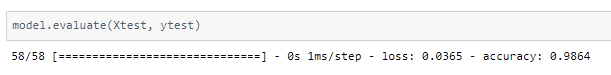
The model achieved around 98% accuracy on the test set.
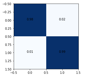
The confusion matrix shows 1% false negatives. In such use cases, it is important to try and reduce false negatives as they may lead to unmonitored seizure episodes putting the patient at risk.
It is important to note that good results, if not the best can be achieved with an unbalanced dataset too. But a wider sample of seizure activity data would result in a better model.
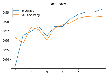
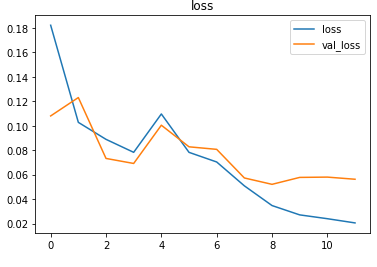
The metrics
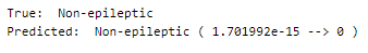
Predictions
Let’s perform predictions on random test data samples —
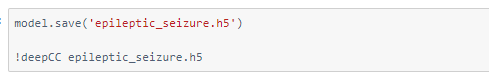
deepC
deepC library, compiler, and inference framework are designed to enable and perform deep learning neural networks by focussing on features of small form-factor devices like micro-controllers, eFPGAs, CPUs, and other embedded devices like raspberry-pi, odroid, Arduino, SparkFun Edge, RISC-V, mobile phones, x86 and arm laptops among others.
Compiling the model using deepC —
Head over to the cAInvas platform (link to notebook given earlier) and check out the predictions by the .exe file!
Credits: Ayisha D
Also Read: Sonar data — Mines vs Rocks — on cAInvas