In a regression problem, we aim to predict the output of a continuous value, like a price or a probability. Contrast this with a classification problem, where we aim to select a class from a list of classes (for example, where a picture contains an apple or an orange, recognizing which fruit is in the picture).

In these types of problems to predict fuel efficiency, we aim to predict a continuous value output, such as a price or a probability. In this article, I will take you through how we can predict Fuel Efficiency with Deep Learning.

Let’s begin !!

Importing the necessary libraries

Let’s import the necessary libraries to get started with this task:

About the dataset

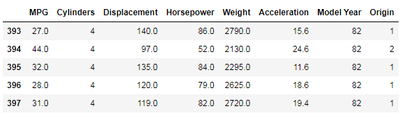
We will be using the classic Auto MPG Dataset and builds a model to predict the fuel efficiency of the late-1970s and early 1980s automobiles. To do this, we’ll provide the model with a description of many automobiles from that time period. This description includes attributes like cylinders, displacement, horsepower, and weight.

The dataset is available from the UCI Machine Learning Repository.

It can be easily downloaded using the following code :

Now, let’s import the data using the pandas package:

Cleaning and Preprocessing of data

The dataset contains a few unknown values.

output :

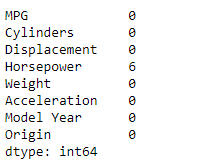
Now let’s drop these rows :

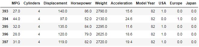
The “origin” column in the dataset is categorical, so to move forward we need to use some one-hot encoding on it:

Now, let’s split the data into training and test sets:

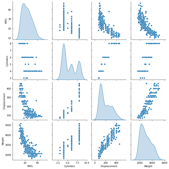
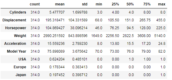
Before training and test to predict fuel efficiency with machine learning, let’s visualize the data by using the seaborn’s pair plot method:

Also, look at the overall statistics:

Now, we will separate the target values from the features in the dataset. This label is that feature that we will use to train the model to predict fuel efficiency:

Normalize the data

It is recommended that you standardize features that use different scales and ranges. Although the model can converge without standardization of features, this makes learning more difficult and makes the resulting model dependent on the choice of units used in the input. We need to do this to project the test dataset into the same distribution the model was trained on:

This normalized data is what we will use to train the model.

Caution: The statistics used to normalize the inputs here (mean and standard deviation) need to be applied to any other data that is fed to the model, along with the one-hot encoding that we did earlier. That includes the test set as well as live data when the model is used in production.

Build The Model

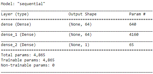
Let’s build our model. Here, I will use the sequential API with two hidden layers and one output layer that will return a single value. The steps to build the model are encapsulated in a function, build_model since we will be creating a second model later :

Use the .summary method to print a simple description of the model :

Now, before training the model to predict fuel efficiency let’s tray this model in the first 10 samples:

output : 
array([[ 0.22689067],
       [ 0.05828134],
       [ 0.2640698 ],
       [ 0.13235056],
       [ 0.41513422],
       [ 0.0909472 ],
       [ 0.47577205],
       [-0.11234067],
       [ 0.24470758],
       [ 0.541355  ]], dtype=float32)

Training Model To Predict Fuel Efficiency

Now, let’s train the model to predict fuel efficiency:

Now, let’s visualize the model training:

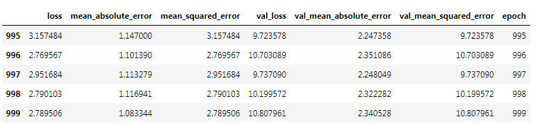
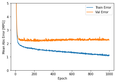
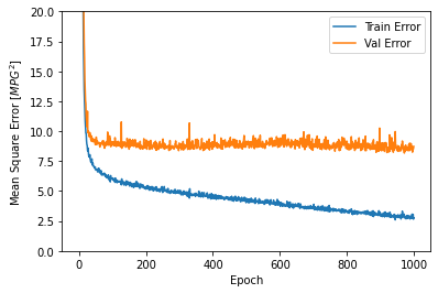
This graph represents a little improvement or even degradation in validation error after about 100 epochs. Now, let’s update the model.fit method to stop training when the validation score does not improve. We’ll be using an EarlyStopping callback that tests a training condition for each epoch. If a set number of epochs pass without showing improvement, automatically stop training:

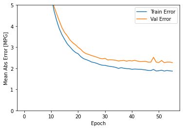
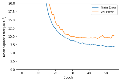
The graph shows that on the validation set, the average error is usually around +/- 2 MPG.

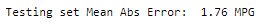
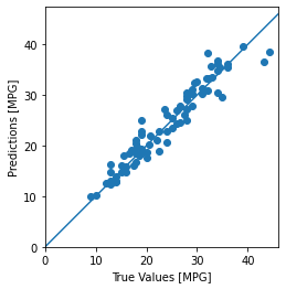
Let’s see how the model generalizes using the test set, which we didn’t use when training the model. This shows how well it is expected that model to predict when we use it in the real world:

Now, let’s make predictions on the model to predict fuel efficiency:

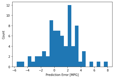
Let’s take a look at the error distribution:

Conclusion :

• Mean Squared Error (MSE) is a common loss function used for regression problems (different loss functions are used for classification problems).
• Similarly, evaluation metrics used for regression differ from classification. A common regression metric is the Mean Absolute Error (MAE).
• When numeric input data features have values with different ranges, each feature should be scaled independently to the same range.
• If there is not much training data, one technique is to prefer a small network with few hidden layers to avoid overfitting.
• Early stopping is a useful technique to prevent overfitting.

Implementation of the project on cainvas here.

Credit: Jeet Chawla