
Introduction
In this project, we will examine the data and build a deep neural network that will classify glass based upon certain features.
Data Source
The data is available publicly over the Kaggle from here you can easily download.
About data
The purpose of the dataset is predict the class of the Glass based upon the given features there’re around 9 features (Id number, RI, Na, Mg, Al, Si, K, Ca, Ba) In which all the columns except the Id columns plays an important role in determining the type of the Glass which also our target variable.
There are 7 types of glasses are in the description provided about the dataset but in a dataset of glasses we don’t have data about type 4 glass each type of glass has it’s own name but in a data the target variable in numbered from 1 to 7. So, based upon the available features we have to predict the target variable (type of glass).
Let’s begin !!
Importing the necessary libraries
Let’s import the necessary libraries to get started with this task:
Reading the CSV file of the dataset
Pandas read_csv() function imports a CSV file (in our case, ‘glass.csv’) to DataFrame format :
Examining the Data
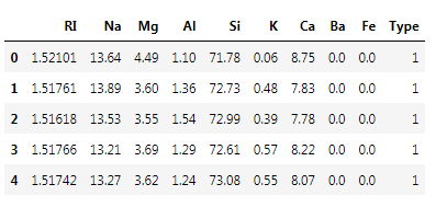
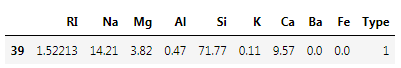
After importing the data, to learn more about the dataset, we’ll use .head() .info() and .describe() methods.
The .head() method will give you the first 5 rows of the dataset. Here is the output:
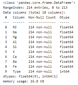
The .info() method will give you a concise summary of the DataFrame. This method will print the information about the DataFrame including the index dtype and column dtypes, non-null values, and memory usage. Here is the output:
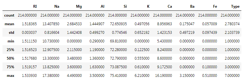
Data summary is one of the useful operation for dataframes which gives us the count, Mean, Standard Deviation along with 5 number summary about the features of the data.
The 5 number summary contain:
- Min
- Q1
- Median
- Q3
- Max
so describe function return the 5 number summary along with other statistical methods like standard deviation, Count and Mean
Here is the output :
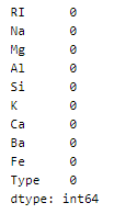
Null Check
There’s is no null value in a dataset.
Here is the output :
Duplicate Check
Let us check the duplicate values :
Here is the output :
Dropping Duplicate
There’re multiple ways to deal with the duplicate records but we have adopted the approach by keeping the last rows and drooping the rows which occurred first in the dataset.
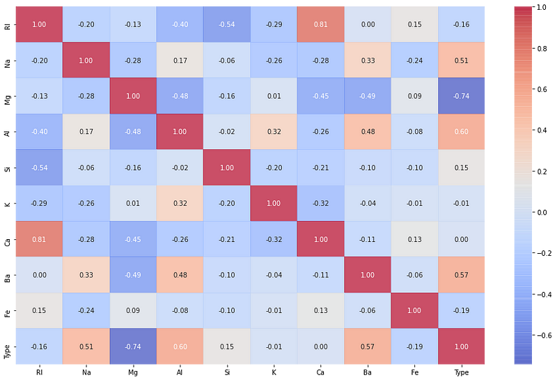
Pairplot
Pairplot shows the relations pairwise among features. Each of the features is plot along grid of axis, So each feature is plotted along the rows as well as along the column.
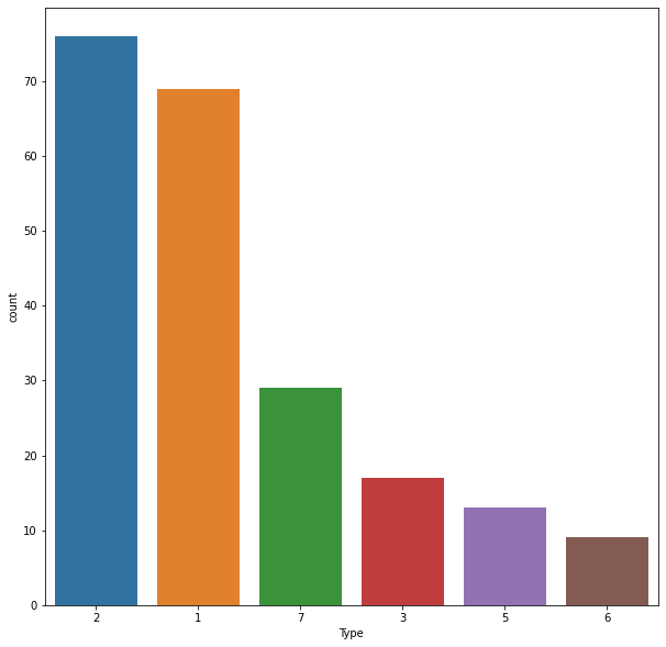
Classes Distribution
The distribution of the Glass type dataset which shows the distribution of each type of glass in a dataset that how many times the particular glass is occurred in a dataset. The distribution shows us that the data is imbalanced.
Data Manipulation
We have separated the features and target variables all the independent variables are stored in X variable where the dependent variable is stored in y variables. The independent variables are normalized by using the normalize function from Keras.Util API of Keras.
Normalization can also be performed by using the Scikit-Learn API of Standard-Scaler or Min-Max-Scaler or Robust-Scaler there’re a lot of methods to deal with this.
Why normalization?
Usually the normalization is performed to bring down all the features on the same scale. By brining down all the features to same scale benefit is that model treat each feature as same.
Class Balancing
As above from Distribution of class we can see that the classes are imbalance so if we develop the model of unbalance dataset the model will bias towards the class containing most of the samples so dealing with imbalance classes will help in developing fair model.
Data Preparation
We will be using 80% of our dataset for training purposes and 20% for testing. It is not possible for us to manually split our dataset also we need to split the dataset in a random manner.
To help us with this task, we will be using a SciKit library named train_test_split. We will be using 80% of our dataset for training purposes and 20% for testing.
X_train : (364, 9)
y_train : (364, 8)
X_test : (92, 9)
y_test : (92, 8)
Building the Neural Network
A Sequential() the function is the easiest way to build a model in Keras. It allows you to build a model layer by layer. Each layer has weights that correspond to the layer the follows it. We use the add() function to add layers to our model.
Fully connected layers are defined using the Dense class. We can specify the number of neurons or nodes in the layer as the first argument, and specify the activation function using the activation argument.
We will use the rectified linear unit activation function referred to as ReLU on the first two layers and the Softmax function in the output layer.
ReLU is the most commonly used activation function in deep learning models. The function returns 0 if it receives any negative input, but for any positive value x it returns that value back. So it can be written as f(x)=max(0,x).
We will also use Dropout and Batch Normalization techniques.
Dropout is a technique where randomly selected neurons are ignored during training. They are “dropped out” randomly. This means that their contribution to the activation of downstream neurons is temporally removed on the forward pass and any weight updates are not applied to the neuron on the backward pass.
Batch Normalization is a technique that is designed to automatically standardize the inputs to a layer in a deep learning neural network.
e.g. We have four features having different units after applying batch normalization it comes in a similar unit.
The softmax function is used as the activation function in the output layer of neural network models that predict a multinomial probability distribution.
Let’s build it :
Compile the Model
Now that the model is defined, we can compile it. We must specify the loss function to use to evaluate a set of weights, the optimizer is used to search through different weights for the network and any optional metrics we would like to collect and report during training.
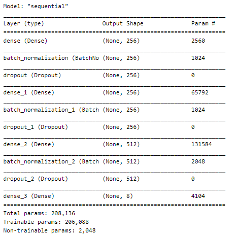
Model Summary
Let’s see our model’s summary :
Now, let’s fit the model :
We have defined our model and compiled it ready for efficient computation.
...
Epoch 395/400
12/12 [==============================] - 0s 3ms/step - loss: 0.5346 - acc: 0.7445 - val_loss: 0.4566 - val_acc: 0.8043
Epoch 396/400
12/12 [==============================] - 0s 3ms/step - loss: 0.4961 - acc: 0.7720 - val_loss: 0.4520 - val_acc: 0.8043
Epoch 397/400
12/12 [==============================] - 0s 3ms/step - loss: 0.5446 - acc: 0.7418 - val_loss: 0.4637 - val_acc: 0.7717
Epoch 398/400
12/12 [==============================] - 0s 4ms/step - loss: 0.5426 - acc: 0.7555 - val_loss: 0.4137 - val_acc: 0.7935
Epoch 399/400
12/12 [==============================] - 0s 3ms/step - loss: 0.5412 - acc: 0.7555 - val_loss: 0.3958 - val_acc: 0.8370
Epoch 400/400
12/12 [==============================] - 0s 3ms/step - loss: 0.5087 - acc: 0.7912 - val_loss: 0.3846 - val_acc: 0.8478
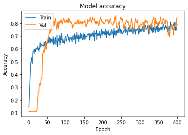
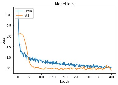
Accuracy and Loss Plots
Let’s define a function for plotting the graphs :
Plotting the curves using the function defined above :
A history object contains all information collected during training.
Graphs :
Model Evaluation
The evaluate() function will return a list with two values. The first will be the loss of the model on the dataset and the second will be the accuracy of the model on the dataset.
[0.38464123010635376, 0.8478260636329651]
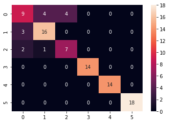
Confusion matrix
Let’s look at the confusion matrix :
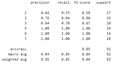
Classification Report
Classification report gives an idea about the class the model has predict orrect and incorrect.
Report :
Making predictions :
array([6, 1, 5, 2, 3, 7, 5, 1, 6, 1, 2, 5, 1, 6, 6, 1, 5, 5, 7, 2, 2, 2,
       3, 2, 3, 7, 2, 7, 2, 3, 6, 3, 7, 2, 7, 2, 5, 5, 2, 2, 6, 2, 7, 2,
       1, 2, 2, 3, 7, 5, 3, 1, 2, 5, 6, 7, 1, 6, 1, 7, 5, 3, 2, 7, 5, 1,
       7, 6, 5, 7, 5, 6, 1, 6, 7, 7, 3, 6, 7, 2, 6, 5, 6, 1, 3, 7, 7, 2,
       1, 2, 1, 3])
We have successfully created our model to classify glass using Deep Neural Network.
Implementation of the project on cainvas here.
Credit: Jeet Chawla
Also Read: Insect Classification