Assess the quality of glass based on derived features using neural networks.

The quality of glass refers to its transparency, heat resistance, stability, etc. It depends on many features such as thickness, composition, luminosity, and many others.
A variation in its composition can define changes in the quality of glass, thus defining how and where it is to be used.
Here, we use deep neural networks to categorize glass samples based on their features into 2 classes.
Implementation of the idea on cAInvas — here!
The dataset
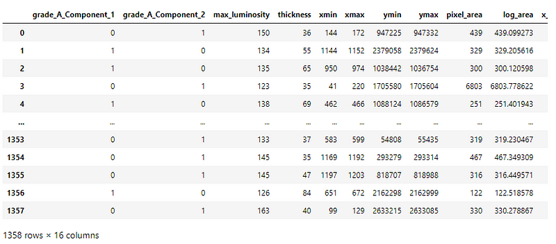
The dataset is a CSV file with 15 feature categories for each sample. There are 2 categories of glass samples — 1 and 2.
Preprocessing
Removing the redundant features
Let us look at the correlation between the feature categories —
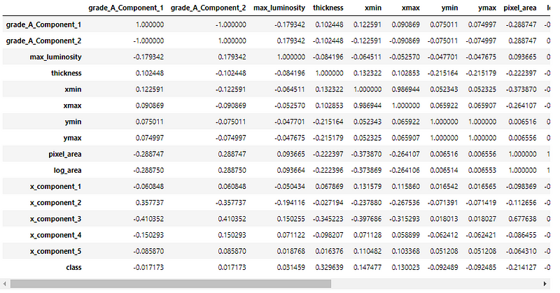
As we can see, there are certain pairs of columns with high correlation (both negative and positive). The sign of the value determines the kind of proportionality between the attributes — positive indicates a direct relation, and negative indicates an indirect relation. The higher the value of the correlation, the higher is the proportionality (direct or inverse) between the pair of attributes.
Removing the columns with a high correlation value reduces the number of attributes, decreasing redundancy in the dataset.
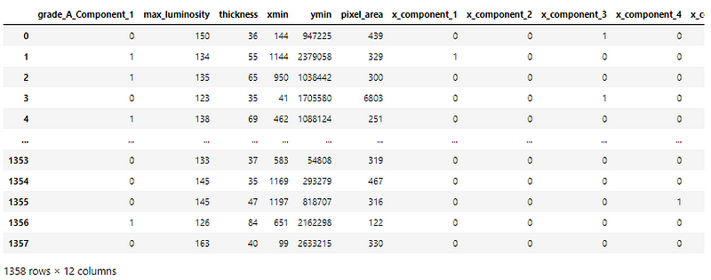
The number of columns has been reduced from 16 to 12. The 4 columns removed are —
- grade_A_Component_2 (inverted grade_A_component_1)
- xmax and ymax are very closely related to xmin and ymin respectively
- log area is directly related to pixel_area
Balancing the dataset
A peek into the distribution of class values among categories —
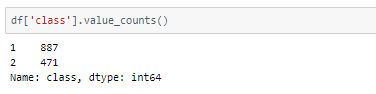
It is an unbalanced dataset. In order to balance the dataset, there are two options,
- upsampling — resample the values to make their count equal to the class label with the higher count (here, 887).
- downsampling — pick n samples from each class label where n = number of samples in class with least count (here, 471)
Here, we will be upsampling.
There are now 887 samples of each category in the dataset.
Renaming the classes
Since this is a binary classification problem, we will rename samples belonging to class 2 as class 0, thus making the two categories for classification 0 and 1.
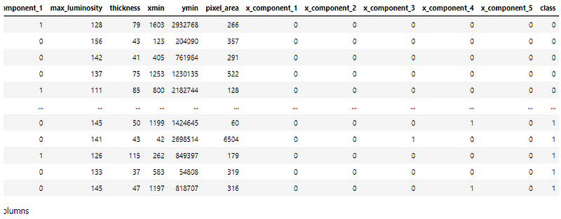
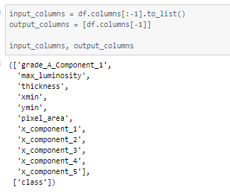
Defining the input and output columns for use later.
Train-validation-test split
Using an 80–10–10 ratio to split the data frame into train-validation-test sets. These are then divided into X and y (input and output) for further processing.
Scaling the values
The range of attribute values is not the same across the dataset. This may result in certain attributes being weighted higher than others. The range of values across all attributes are scaled to [0, 1].
The MinMaxScaler function of the sklearn.preprocessing module is used to implement this concept. The instance is fit on the training data and used to transform the train, validation, and test data.
The model
The model is a simple one with 4 Dense layers, 3 of which have ReLU activation functions and the last one has a Sigmoid activation function that outputs a value in the range [0, 1].
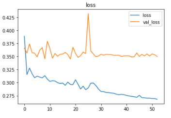
As it is a binary classification problem, the model is compiled using the binary cross-entropy loss function. The Adam optimizer is used and the accuracy of the model is tracked over epochs.
The EarlyStopping callback function monitors the validation loss and stops the training if it doesn’t decrease for 10 epochs continuously. The restore_best_weights parameter ensures that the model with the least validation loss is restored to the model variable.
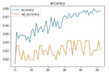
The model was trained first with a learning rate of 0.01 and then with a learning rate of 0.001.
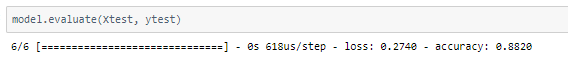
The model achieved an accuracy of ~88% on the test set.
Plotting a confusion matrix to understand the results better —
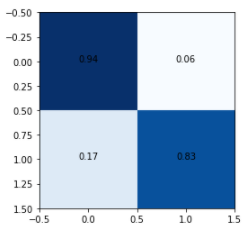
A larger dataset would help in achieving a higher test set accuracy.
The metrics
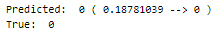
Prediction
Let’s perform predictions on random test data samples —
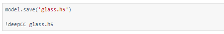
deepC
deepC library, compiler, and inference framework are designed to enable and perform deep learning neural networks by focussing on features of small form-factor devices like micro-controllers, eFPGAs, CPUs, and other embedded devices like raspberry-pi, odroid, Arduino, SparkFun Edge, RISC-V, mobile phones, x86 and arm laptops among others.
Compiling the model using deepC —
Head over to the cAInvas platform (link to notebook given earlier) and check out the predictions by the .exe file!
Credits: Ayisha D