
You’ll want to evaluate almost every model you ever build. In most (though not all) applications, the relevant measure of model quality is predictive accuracy. In other words, will the model’s predictions be close to what actually happens.
Many people make a huge mistake when measuring predictive accuracy. They make predictions with their training data and compare those predictions to the target values in the training data. You’ll see the problem with this approach and how to solve it.
Before starting, I would like to give an overview of how to structure any deep learning project.
- Preprocess and load data- As we have already discussed data is the key for the working of a neural network and we need to process it before feeding it to the neural network. In this step, we will also visualize data which will help us to gain insight into the data.
- Define model- Now we need a neural network model. This means we need to specify the number of hidden layers in the neural network and their size, the input, and output size.
- Loss and optimizer- Now we need to define the loss function according to our task. We also need to specify the optimizer to use with the learning rate and other hyperparameters of the optimizer.
- Fit model- This is the training step of the neural network. Here we need to define the number of epochs for which we need to train the neural network.
After fitting the model, we can test it on test data to check whether the case of overfitting. We can save the weights of the model and use it later whenever required.
Importing the Libraries and Loading the data
Data processing
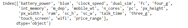
We will use simple data of mobile price range classifier. The dataset consists of 20 features and we need to predict the price range in which the phone lies. These ranges are divided into 4 classes. The features of our dataset include the columns as follows:
Before feeding data to our neural network we need it in a specific way so we need to process it accordingly. The preprocessing of data depends on the type of data.
Our dataset looks like.
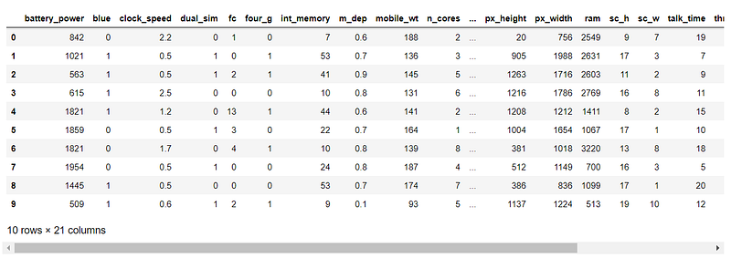
This code as discussed in the python module will make two arrays X and y. X contains features and y will contain classes.
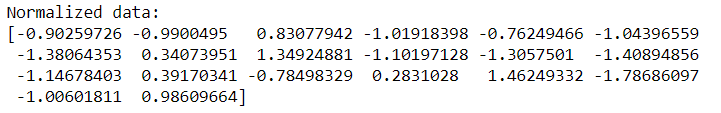
This step is used to normalize the data. Normalization is a technique used to change the values of an array to a common scale, without distorting differences in the ranges of values. It is an important step and you can check the difference in accuracies on our dataset by removing this step.
It is mainly required in case the dataset features vary a lot as in our case the value of battery power is in the 1000’s and clock speed is less than 3. So if we feed unnormalized data to the neural network, the gradients will change differently for every column and thus the learning will oscillate.
The X will now be changed to this form:
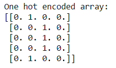
The next step is to one-hot encode the classes. One hot encoding is a process to convert integer classes into binary values. Consider an example, let’s say there are 3 classes in our dataset namely 1,2, and 3. Now we cannot directly feed this to the neural network so we convert it into the form:
- 1- 1 0 0
- 2- 0 1 0
- 3- 0 0 1
Now there is one unique binary value for the class. The new array formed will be of shape (n, number of classes), where n is the number of samples in our dataset. We can do this using a simple function by sklearn:
https://gist.github.com8226792d36194c2293bf39eb4ae53c3e
Our dataset has 4 classes so our new label array will look like this:
Now our dataset is processed and ready to feed in the neural network.
Generally, it is better to split data into training and testing data. Training data is the data on which we will train our neural network. Test data is used to check our trained neural network. This data is totally new for our neural network and if the neural network performs well on this dataset, it shows that there is no overfitting.
This will split our dataset into training and testing. Training data will have 90% samples and test data will have 10% samples. This is specified by the test_size argument.
Now we are done with the boring part and let’s build a neural network.
Building Neural Network
Keras is a simple tool for constructing a neural network. It is a high-level framework based on TensorFlow, theano, or cntk backends.
In our dataset, the input is of 20 values and output is of 4 values. So the input and output layer is of 20 and 4 dimensions respectively.
In our neural network, we are using two hidden layers of 16 and 12 dimensions.
Now I will explain the code line by line.
Sequential specifies to Keras that we are creating a model sequentially and the output of each layer we add is input to the next layer we specify.
model.add is used to add a layer to our neural network. We need to specify as an argument what type of layer we want. The Dense is used to specify the fully connected layer. The arguments of Dense are output dimension which is 16 in the first case, input dimension which is 20 for input dimension and the activation function to be used which is relu in this case.
The second layer is similar, we don’t need to specify the input dimension as we have defined the model to be sequential so Keras will automatically consider the input dimension to be the same as the output of the last layer i.e 16.
In the third layer(output layer) the output dimension is 4(number of classes). Now as we have discussed earlier, the output layer takes different activation functions and for the case of multiclass classification, it is softmax.
Now we need to specify the loss function and the optimizer. It is done using compile function in Keras.
Here loss is cross-entropy loss as discussed earlier. Categorical_crossentropy specifies that we have multiple classes. The optimizer is Adam. Metrics is used to specify the way we want to judge the performance of our neural network. Here we have specified it to accuracy.
Now we are done with building a neural network and we will train it.
Training model
The training step is simple in Keras. model.fit is used to train it.
Here we need to specify the input data-> X_train, labels-> y_train, number of epochs(iterations), and batch size. It returns the history of model training. History consists of model accuracy and losses after each epoch. We will visualize it later.
Usually, the dataset is very big and we cannot fit complete data at once so we use batch size. This divides our data into batches each of size equal to batch_size. Now only this number of samples will be loaded into memory and processed. Once we are done with one batch it is flushed from memory and the next batch will be processed.
Now we have started the training of our neural network.
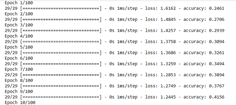
It will take around a minute to train. And after 100 epochs the neural network will be trained. The training accuracy is reached 93.5 % so our model is trained.
Now we can check the model’s performance on test data:
This step is inverse one hot encoding process. We will get integer labels using this step. We can predict on test data using a simple method of Keras, model. predict(). It will take the test data as input and will return the prediction outputs as softmax.
We get an accuracy of 95.5%.
We can use test data as validation data and can check the accuracies after every epoch. This will give us an insight into overfitting at the time of training only and we can take steps before the completion of all epochs. We can do this by changing the fit function as:
Now the training step output will also contain validation accuracy.
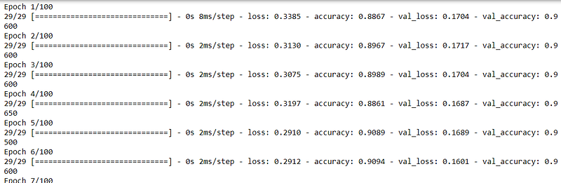
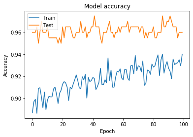
Our model is working fine. Now we will visualize training and validation losses and accuracies.
Plotting the graph for Model Accuracy
Plotting graph for Model Loss

So, this is all about this project.
This is project is working completely fine with the perfect accuracies.
You can download the notebook from here.
Credit: Bhupendra Singh Rathore
Also Read: Fingerprint pattern classification using Deep Learning