Introduction

Blood is a constantly circulating body fluid which delivers nutrients and oxygens to the cells and aids in the transport of metabolic by-products away from the cells. It is one of the most vital components of the human body and multiple functionalities of the body organs rely on healthy blood. The healthiness of blood can be assessed by analyzing the healthiness of the various constituents of blood.

The human blood consists of blood cells suspended in a liquid portion known as the plasma. The blood cells constitute about 45% of the blood volume, while the plasma constitutes the remaining 55%. The blood cells are of three types that include red blood cells, white blood cells and the platelets.

The diagnosis of blood-based diseases often involves identifying and characterizing patient blood samples. Automated methods to detect and classify blood cell subtypes will facilitate in faster diagnosis and better patient outcomes.

In this article, our main focus will revolve around the classification of the different types of white blood cells using deep learning techniques on the Cainvas platform.

The dataset

The dataset used in this article can be fetched from here.

The dataset contains 12500 augmented colored images of blood cells in JPEG format. There are 4 different classes of White blood cells — Eosinophil, Lymphocyte, Monocyte, and Neutrophil, in the dataset.

In this article, we will use Tensorflow — an opensource software library that provide tools and resources to create machine learning algorithms, and Keras — an interface for the Tensorflow library for developing deep learning models , to create a convolutional neural network and try to accurately predict the classes of the white blood cells from the images of the blood samples.

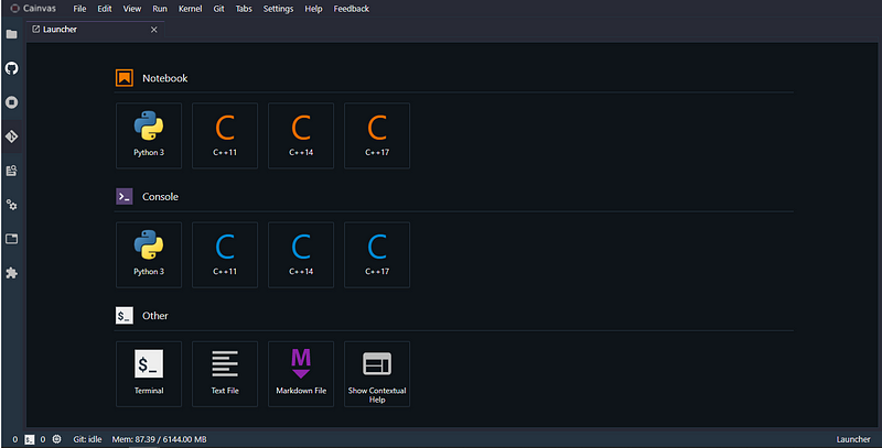
The entire code will be written on the Cainvas platform’s Notebook Server for better performance as well as scaling the model later to use it in EDGE devices.

Setting Up the Platform

You can create an account on the Cainvas website here.

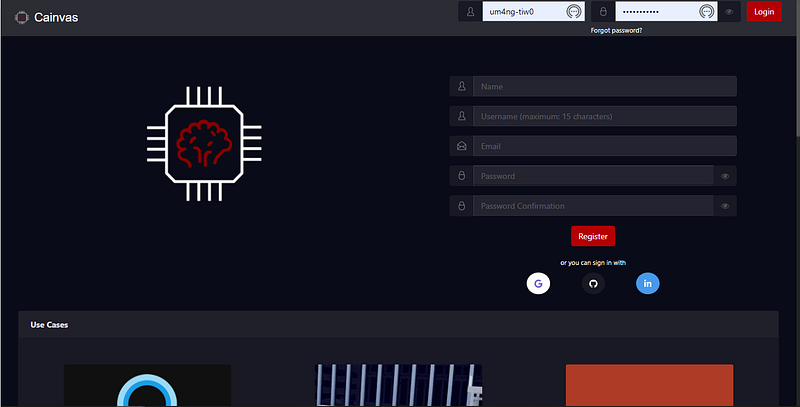
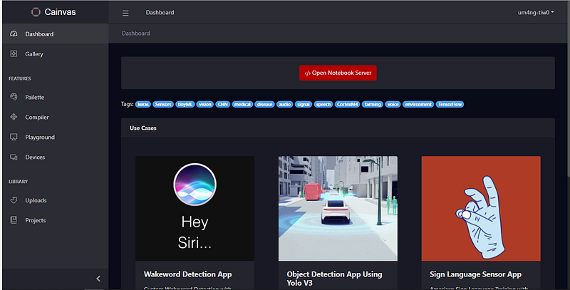
After successful creation of an account, login to the platform and go to the Dashboard section to open the Notebook Server.

Importing the necessary libraries

We will use some commonly used libraries like Numpy and Matplotlib. We will use OpenCV2 and Matplotlib to access the images and display it in the notebook.

Other imports include Tensorflow and Keras to create the convolutional neural network and perform preprocessing of the data to perform training on it.

Loading the dataset

Cainvas platform allows us to upload datasets on the platform which facilitates ease of use. These datasets can be then easily loaded on to the notebook and used with enough flexibility to create the model without any hassle.

In order to upload your dataset, you can head to the Pailette section which allows uploading of files, images, videos and even sensor data.

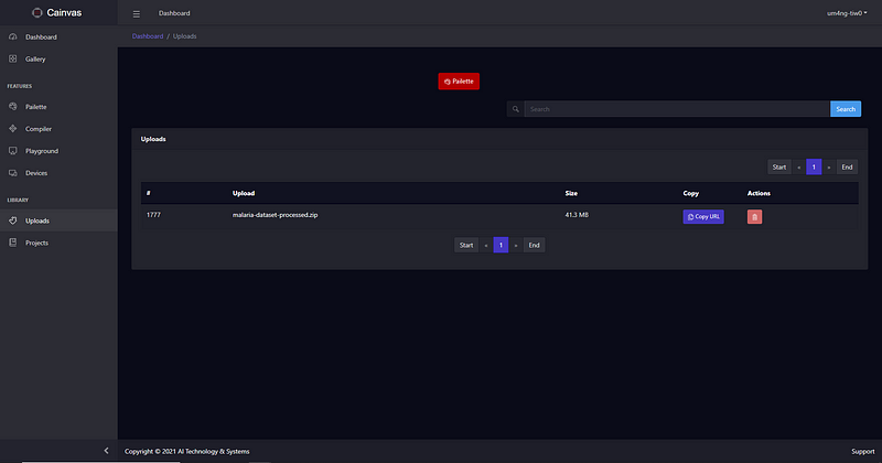
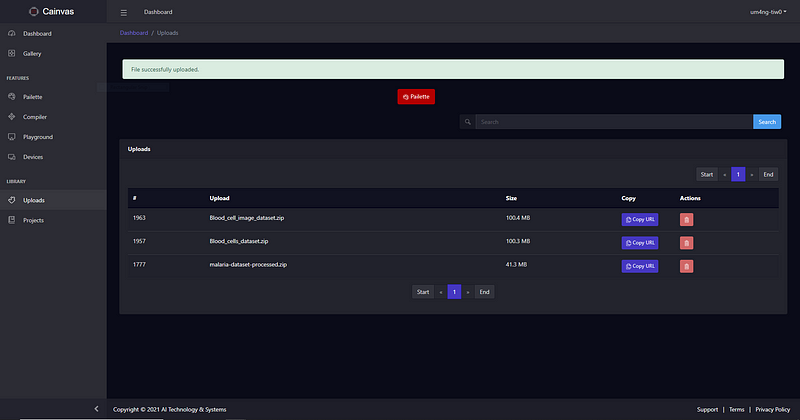
We will upload the dataset as a zip file in this article. The URL of the uploaded file can be obtained after the upload and used in the notebook to fetch it. To view the uploaded files just click on the Uploads sections. Click on the Copy URL button to copy the URL of the file.

We can use the URL with !wget command to load it in our notebook. We can then unzip the zip file in quiet mode using!unzip -qo filename.zip

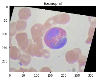
We can access an image to check if the dataset has been loaded successfully.

Preparing the data

The training data is present inside four folders — Eosinophil, Lymphocyte, Monocyte, and Neutrophil, representing the four classes of the white blood cells. We will use the ImageDataGenerator offered by Keras to prepare the data and get appropriate labels pertaining to the folder structure. The generator also provides us the flexibility of creating train and validation split sets from the entire training dataset.

We can now check the labels fetched through the folder structure of our Training data.

array([[0., 1., 0., 0.],
       [0., 1., 0., 0.],
       [0., 0., 1., 0.],
       [1., 0., 0., 0.],
       [0., 0., 1., 0.],
       [0., 0., 0., 1.],
       [0., 1., 0., 0.],
       [0., 0., 0., 1.],
       [0., 1., 0., 0.],
       [1., 0., 0., 0.],
       [1., 0., 0., 0.],
       [0., 0., 0., 1.],
       [0., 0., 1., 0.],
       [1., 0., 0., 0.],
       [1., 0., 0., 0.],
       [1., 0., 0., 0.]], dtype=float32)

We receive one hot encoded vectors due to the categorical nature of the data. The index position of 1s indicate the corresponding class of the white blood cell in the image.

Creating the Model

As mentioned, we will create a Convolutional Neural Network to predict the correct classes of cells from the images. We have used 3 Conv2D layers with MaxPool2D layers after each for the feature extraction from the images.

The activation function used is ReLU. The output layer has only four neurons corresponding to the four classes of the white blood cells, with Softmax activation function.

The model summary for the above created model is as follow:

Model: "sequential_9"
_________________________________________________________________
Layer (type)                 Output Shape              Param #   
=================================================================
conv2d_27 (Conv2D)           (None, 62, 62, 32)        896       
_________________________________________________________________
max_pooling2d_27 (MaxPooling (None, 31, 31, 32)        0         
_________________________________________________________________
conv2d_28 (Conv2D)           (None, 29, 29, 32)        9248      
_________________________________________________________________
max_pooling2d_28 (MaxPooling (None, 14, 14, 32)        0         
_________________________________________________________________
conv2d_29 (Conv2D)           (None, 12, 12, 16)        4624      
_________________________________________________________________
max_pooling2d_29 (MaxPooling (None, 6, 6, 16)          0         
_________________________________________________________________
flatten_9 (Flatten)          (None, 576)               0         
_________________________________________________________________
dense_18 (Dense)             (None, 128)               73856     
_________________________________________________________________
dense_19 (Dense)             (None, 4)                 516       
=================================================================
Total params: 89,140
Trainable params: 89,140
Non-trainable params: 0
_________________________________________________________________

We will use Early Stopping so that our model stops training if the monitored parameter does not change over time. This will make the training process more efficient

Compiling and Training the Model

We will compile the model with Adam as the optimizer and Categorical Crossentropy as the loss function. We will train the model for 100 epochs with the callback. We will store the accuracy, loss, val_accuracy and val_loss at each epoch in the history for plotting meaningful data later.

The last three epochs of the training phase:

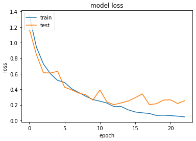
Epoch 21/100
622/622 [==============================] - 15s 24ms/step - loss: 0.0625 - accuracy: 0.9800 - val_loss: 0.2654 - val_accuracy: 0.9095
Epoch 22/100
622/622 [==============================] - 15s 23ms/step - loss: 0.0548 - accuracy: 0.9819 - val_loss: 0.2174 - val_accuracy: 0.9216
Epoch 23/100
622/622 [==============================] - 15s 24ms/step - loss: 0.0460 - accuracy: 0.9869 - val_loss: 0.2545 - val_accuracy: 0.9115

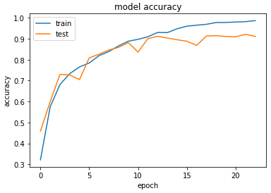
Accuracy & Loss

We will plot the model performance at each epoch during the training phase.

Testing the Model

We will now test the model by evaluating on the unseen test data which contains 54 images distributed in the 4 classes.

4/4 [==============================] - 0s 18ms/step - loss: 0.1172 - accuracy: 0.9661
[0.11723806709051132, 0.9661017060279846]

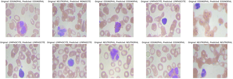
We will now predict the first 10 images in the test data. We will first create more meaningful output from one hot encoded vectors.

ACTUAL: {0: \'EOSINOPHIL\', 1: \'NEUTROPHIL\', 2: \'EOSINOPHIL\', 3: \'LYMPHOCYTE\', 4: \'EOSINOPHIL\', 5: \'LYMPHOCYTE\', 6: \'LYMPHOCYTE\', 7: \'NEUTROPHIL\', 8: \'EOSINOPHIL\', 9: \'NEUTROPHIL\'}

PREDICTIONS: {0: \'EOSINOPHIL\', 1: \'MONOCYTE\', 2: \'EOSINOPHIL\', 3: \'LYMPHOCYTE\', 4: \'EOSINOPHIL\', 5: \'LYMPHOCYTE\', 6: \'LYMPHOCYTE\', 7: \'NEUTROPHIL\', 8: \'EOSINOPHIL\', 9: \'NEUTROPHIL\'}

Visualizing the predictions for better insights

Conclusion

In this article, we saw how to predict the correct class of a given white blood cell image using a convolutional neural network created on the Cainvas Platform. We observed the capabilities of artificial intelligence and a simple use case of how it can be employed to automate healthcare systems.

The Cainvas Platform provides a one stop solution to creating deep learning models which can also be compiled into EDGE device friendly models for using it in your IOT projects. The platform boasts of various other tools and resources to guide you for your next deep learning IOT project.

Notebook Link: Here.

Credit: Umang Tiwari