Use deep learning to identify three types of rice leaf diseases.

Classifying plant species or diseases in plants can sometimes be a challenging task for the human eye, especially for people with limited experience in the field. There is little margin for error allowed when it comes to crops and farming as our very livelihoods depend on it. Thus, we use a deep learning approach to try and minimize this error.
Of the three major crops — rice, wheat and maize — rice is by far the most important food crop for people in low- and lower-middle-income countries. Although rich and poor people alike eat rice in low-income countries, the poorest people consume relatively little wheat and are therefore deeply affected by the cost and availability of rice.
~ Quote ricepedia.org
Diseases in plants occur in different colours, sizes, shapes and each one has its own individual features. Sheath rot, leaf blast, leaf smut, brown spot, and bacterial blight are the most common diseases in rice leaves.
In this article, we will use deep learning to classify images of rice leaf diseases into three categories — Bacterial leaf blight, brown spot, and leaf smut.
The implementation of the idea on cAInvas is here.
The dataset
Citation
Prajapati HB, Shah JP, Dabhi VK. Detection and classification of rice plant diseases. Intelligent Decision Technologies. 2017 Jan 1;11(3):357–73, doi: 10.3233/IDT-170301.
The dataset has 3 folders, each with 40 images of a specific disease type, and is thus a balanced dataset.
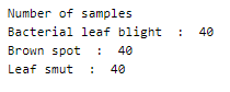
The labels, as mentioned above, are bacterial leaf blight, brown spot, and leaf smut.
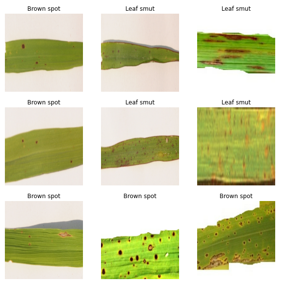
Here is a peek into a few of the dataset images —
Preprocessing
Normalization
The pixel values of these images are integers in the range 0–255. Normalizing the pixel values reduces them to float values in the range [0, 1]. This is done using the Rescaling function of the keras.layers.experimental.preprocessing module.
Normalization helps in faster convergence of the model’s loss function.
Augmentation
The dataset has only 40 images per class. This is not enough data to get good results.
Image data augmentation is a technique to artificially increase the size of the training dataset using techniques like scaling (or resizing), cropping, flipping (horizontal or vertical or both), padding, rotation, translation (movement along x or y-axis). Colour augmentation techniques include adjusting the brightness, contrast, saturation, and hue of the images.
Here, we will implement two image augmentation techniques using functions from the keras.layers.experimental.preprocessing module —
- RandomFlip — randomly flip the images along the directions specified as a parameter (horizontal or vertical or both)
- RandomZoom — random images in the dataset are zoomed 10%.
Feel free to try out other augmentation techniques!
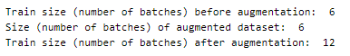
We have now doubled the training data.
The model
We are using transfer learning, which is the concept of using the knowledge gained while solving one problem to solve another problem.
Xception architecture is an extension of the Inception architecture with depthwise separable convolutions replacing the standard Inception modules.
The model’s input is defined to have a size of (256, 256, 3).
The last layer of the Xception model (classification layer) is not included and instead, it is appended with a GlobalAveragePooling layer followed by a Dense layer with softmax activation and as many nodes as there are classes.
The model is configured such that the appended layers are the only trainable part of the entire model. This means that, as the training epochs advance, the weights of nodes in the Xception architecture remain constant.
The model is compiled using Adam optimizer with a learning rate of 0.01.
SparseCategoricalCrossentropy loss of the Keras module is used as the class labels are not one-hot encoded.
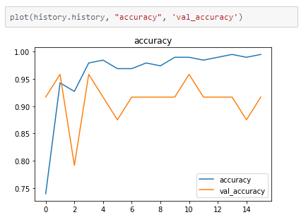
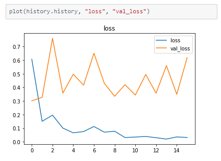
The model’s accuracy on the input data is tracked at the end of every epoch.
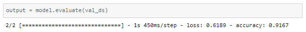
At the end of 16 epochs, we are able to achieve 91.67% accuracy on validation data.
The metrics
Prediction
Let’s look at the validation image along with the model’s prediction —
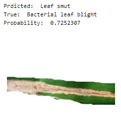
Given that our accuracy was only ~91%…a few mistakes are bound to happen.
deepC
deepC library, compiler, and inference framework are designed to enable and perform deep learning neural networks by focussing on features of small form-factor devices like micro-controllers, eFPGAs, CPUs, and other embedded devices like raspberry-pi, odroid, Arduino, SparkFun Edge, RISC-V, mobile phones, x86 and arm laptops among others.
Compiling the model using deepC —
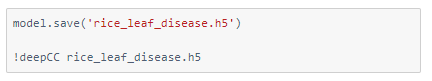
Head over to the cAInvas platform (link to notebook given earlier) to run and generate your own .exe file!
Credits: Ayisha D
Also Read: Disease Classification using Medical MNIST