Using a ConvNet to detect the presence of ships in aerial images taken of the San Francisco Bay

Satellite imagery provides unique insights into various markets, including agriculture, defense and intelligence, energy, and finance. New commercial imagery providers, such as Planet, are using constellations of small satellites to capture images of the entire Earth every day.
This flood of new imagery is outgrowing the ability for organizations to manually look at each image that gets captured, and there is a need for machine learning and computer vision algorithms to help automate the analysis process.
The aim of this ConvNet is to help address the difficult task of detecting the location of large ships in satellite images. Automating this process can be applied to many issues including monitoring port activity levels and supply chain analysis.
This model can be used in more complex frameworks such as the YOLOv3 model and Fast R-CNN models so that multiple ships in the port can be pinpointed with bounding boxes around them.
Dataset
The dataset consists of image chips extracted from Planet satellite imagery collected over the San Francisco Bay and San Pedro Bay areas of California. It includes 4000 80×80 RGB images labeled with either a “ship” or “no-ship” classification.
Image chips were derived from PlanetScope full-frame visual scene products, which are orthorectified to a 3 meter pixel size.
Requirements
- Numpy
- Pandas
- Scikit-image
- Matplotlib
- Tensorflow
- Keras
- Cainvas Notebook Server
Here’s How it Works
- Our input is a training dataset that consists of N images, each labeled with one of 2 different classes.
- Then, we use this training set to train a ConvNet to learn what each of the classes looks like.
- In the end, we evaluate the quality of the classifier by asking it to predict labels for a new set of images that it has never seen before. We will then compare the true labels of these images to the ones predicted by the classifier.
- The model and its weights are then saved for future uses.
We’ll be using the Cainvas platform which provides us with powerful resources over the cloud to deliver robust models which are also available for future deployment on EDGE devices.
Code
Let’s get started with the code.
We’ll be using matplotlib to plot the images and the labels. Tensorflow and Keras are one of the most commonly used deep learning frameworks and we’ll be using them to create our ConvNet and engineer our model.
Loading the dataset
The images from the dataset are loaded into NumPy arrays, with labels [0,1] corresponding to the classes no-ship and ship. The data was loaded into NumPy arrays as data augmentation and upsampling/downsampling is easier to perform.
Exploratory Data Analysis
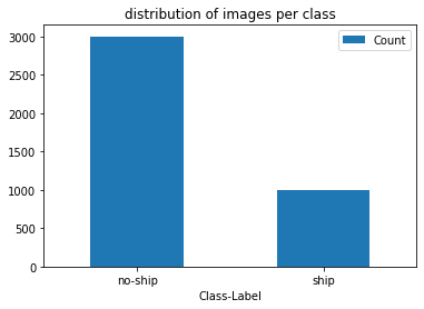
Here we’ll be performing a simple EDA of the dataset to determine whether the classes are imbalanced or not using a bar plot.
Data Augmentation
The images present in the ship class are augmented and then stored in the dataset, so that there is an equal representation of the classes.
The current ratio of classes is 1:3, meaning that for every image present in the ship class there are 3 images present in the no-ship class. This will be countered by producing 2 augmented images per original image of the ship class. This will make the dataset balanced.
Then the labels NumPy array is one hot encoded using to_categorical from Keras. This removes any unnecessary bias in the dataset, by keeping the class at equal footing, with respect to labels.
Splitting the data
Instead of using train_test_split the images and labels arrays are randomly shuffled using the same seed value set at 42. This allows the images and their corresponding labels to remain linked even after shuffling.
This method allows the user to make all 3 datasets. The training and validation dataset is used for training the model while the testing dataset is used for testing the model on unseen data. Unseen data is used for simulating real-world prediction, as the model has not seen this data before. It allows the developers to see how robust the model is.
The data has been split into –
- 70% — Training
- 20% — Validation
- 10% — Testing
Model Architecture
Our model structure consists of four Conv2D layers including the input layer with a 2×2 MaxPool2D pooling layer each followed by a dense layer of 64 neurons and one dense layer of 128 neurons each with a ReLU activation function and the last layer with 2 neurons and the softmax activation function for making our class predictions.
Model: "sequential"
_________________________________________________________________
Layer (type)                 Output Shape              Param #
=================================================================
zero_padding2d (ZeroPadding2 (None, 58, 58, 3)         0
_________________________________________________________________
conv2d (Conv2D)              (None, 56, 56, 16)        448
_________________________________________________________________
batch_normalization (BatchNo (None, 56, 56, 16)        64
_________________________________________________________________
conv2d_1 (Conv2D)            (None, 54, 54, 32)        4640
_________________________________________________________________
batch_normalization_1 (Batch (None, 54, 54, 32)        128
_________________________________________________________________
max_pooling2d (MaxPooling2D) (None, 27, 27, 32)        0
_________________________________________________________________
dropout (Dropout)            (None, 27, 27, 32)        0
_________________________________________________________________
conv2d_2 (Conv2D)            (None, 23, 23, 32)        25632
_________________________________________________________________
batch_normalization_2 (Batch (None, 23, 23, 32)        128
_________________________________________________________________
max_pooling2d_1 (MaxPooling2 (None, 11, 11, 32)        0
_________________________________________________________________
dropout_1 (Dropout)          (None, 11, 11, 32)        0
_________________________________________________________________
conv2d_3 (Conv2D)            (None, 9, 9, 64)          18496
_________________________________________________________________
batch_normalization_3 (Batch (None, 9, 9, 64)          256
_________________________________________________________________
max_pooling2d_2 (MaxPooling2 (None, 4, 4, 64)          0
_________________________________________________________________
dropout_2 (Dropout)          (None, 4, 4, 64)          0
_________________________________________________________________
flatten (Flatten)            (None, 1024)              0
_________________________________________________________________
dense (Dense)                (None, 64)                65600
_________________________________________________________________
dropout_3 (Dropout)          (None, 64)                0
_________________________________________________________________
dense_1 (Dense)              (None, 128)               8320
_________________________________________________________________
dense_2 (Dense)              (None, 2)                 258
=================================================================
Total params: 123,970
Trainable params: 123,682
Non-trainable params: 288
_________________________________________________________________
I defined checkpoints specifying when to save the model and implemented early stopping to make the training process more efficient.
I have used Adam as the optimizer as it was giving much better results. I have used binary cross-entropy as the loss function for our model since there are only 2 classes. I trained the model for 50 iterations. However, you’re free to use a number of different parameters to your liking as long as the accuracy of the predictions doesn’t suffer.
This is a function to plot loss and accuracy which we will get after training the model. The model was saved and the results were plotted using the defined function.
Results
Loss/Accuracy vs Epoch
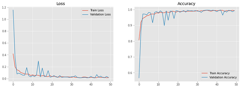
The model reached a validation accuracy of roughly 70% which is quite decent considering the size of the dataset and the fact that we are keeping the model lightweight for deployment.
Predictions
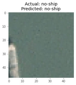
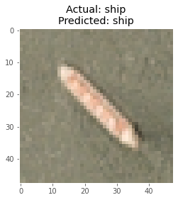
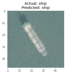
I took a batch of 8 images from the test images and plotted them with the corresponding true and predicted labels after making the predictions using the model.
Here are some of the predictions made by the model :
Conclusion
In this article, I’ve demonstrated how a ConvNet built from scratch can be used to detect ships in ports from aerial imagery using deep learning. This simple use-case can be used as a module in more complex frameworks for achieving object detection where the ships can be detected and marked out from a single scene image.
Notebook Link: Here.
Credit: Ved Prakash Dubey
Also Read: Blood Cell classification using Deep Learning on Cainvas Platform