
Introduction
Neural Network is a programming paradigm inspired from the biological neurons in the human body. The neural networks are a set of algorithms that are modeled after the human brain, that are designed to capture patterns from the observational data.
Today neural networks are used in a plethora of applications, from simple object detection to bigger applications like self-driving vehicles.
The Fashion MNIST Dataset
Fashion-MNIST is a dataset of Zalando’s article images — consisting of a training set of 60,000 examples and a test set of 10,000 examples. Each example is a 28×28 grayscale image, associated with a label from 10 classes. Zalando intends Fashion-MNIST to serve as a direct drop-in replacement for the original MNIST dataset for benchmarking machine learning algorithms. It shares the same image size and structure of training and testing splits.
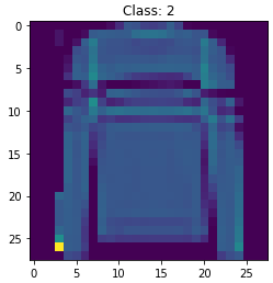
Each image in the dataset is 28 pixels in height and 28 pixels in width, for a total of 784 pixels in total. Each pixel has a single pixel-value associated with it, indicating the lightness or darkness of that pixel, with higher numbers meaning darker. This pixel-value is an integer between 0 and 255.
The following are the clothing items and their corresponding classes:
- Class 0: T-shirt/top
- Class 1: Trouser
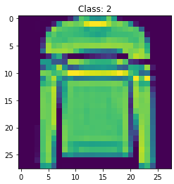
- Class 2: Pullover
- Class 3: Dress
- Class 4: Coat
- Class 5: Sandal
- Class 6: Shirt
- Class 7: Sneaker
- Class 8: Bag
- Class 9: Ankle Boot
In this article, we will use Tensorflow — an opensource software library that provide tools and resources to create machine learning algorithms, and Keras — an interface for the Tensorflow library for developing deep learning models, to create a neural network and try to accurately classify the images to their corresponding correct classes.
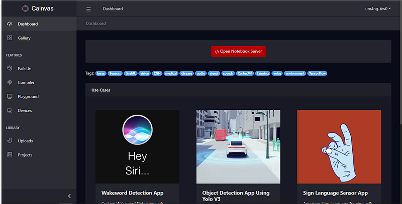
The entire code will be written on the Cainvas platform’s Notebook Server for better performance as well as scaling the model later to use it in EDGE devices.
Setting Up the Platform
You can create an account on the Cainvas website here.
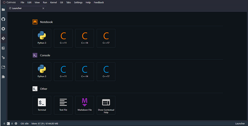
Click on the Python 3 option under the Notebook section to create a new Python notebook.
Importing the necessary libraries
We will use some commonly used libraries like Numpy and Matplotlib. Matplotlib will be used to plot images and graphs so that we can observe the neural network performance while training and testing.
We will also import Keras to create our neural network.
Loading the Dataset
The dataset can be loaded directly from tensorflow.keras.dataset. The training shape is (60000,28,28) and the test shape is (10000,28,28), i.e. the training set contains 60000 images of 28×28 dimension and the test set contains 10000 images of 28×28 dimension.
Normalizing the data
We will preprocess the data by normalizing it. The pixel value of the images range from 0 to 255. This feature range may consume more time while converging towards the minimum. Therefore, we will normalize the data to bring these values between 0 and 1. This smoothens the training process and yields better accuracy in lesser time.
Neural Network Architecture
We will use a 4-layer neural network in this article to perform the classification of the images.
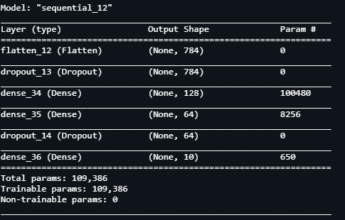
The flatten layer will flatten the 28×28 image to 784. The second layer is a Dense layer with ReLU as the activation function. The last layer has 10 units corresponding to the 10 classes of clothing of the dataset. The last layer uses the Softmax as the activation function which is well suited for categorical data. The dropouts have been used to prevent overfitting of the network
Model: “sequential_12”
_________________________________________________________________
Layer (type) Output Shape Param #
=================================================================
flatten_12 (Flatten) (None, 784) 0
_________________________________________________________________
dropout_13 (Dropout) (None, 784) 0
_________________________________________________________________
dense_34 (Dense) (None, 128) 100480
_________________________________________________________________
dense_35 (Dense) (None, 64) 8256
_________________________________________________________________
dropout_14 (Dropout) (None, 64) 0
_________________________________________________________________
dense_36 (Dense) (None, 10) 650
=================================================================
Total params: 109,386
Trainable params: 109,386
Non-trainable params: 0
_________________________________________________________________
Compiling and Training the model
We will compile the model with the following parameters.
The optimizer used here is Adam and the loss function is the Sparse categorical crossentropy.
We will train the model using the following parameters. We will use 0.33 of the data for validation at each epoch and train the model for 20 epochs.
We will store the accuracy, loss, val_accuracy, and val_loss at each epoch in the history for plotting meaningful data later.
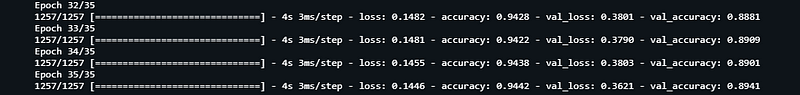
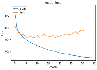
Epoch 33/35
1257/1257 [==============================] - 4s 3ms/step - loss: 0.1481 - accuracy: 0.9422 - val_loss: 0.3790 - val_accuracy: 0.8909
Epoch 34/35
1257/1257 [==============================] - 4s 3ms/step - loss: 0.1455 - accuracy: 0.9438 - val_loss: 0.3803 - val_accuracy: 0.8901
Epoch 35/35
1257/1257 [==============================] - 4s 3ms/step - loss: 0.1446 - accuracy: 0.9442 - val_loss: 0.3621 - val_accuracy: 0.8941
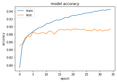
Accuracy and Loss
We will plot the model performance at each epoch during the training phase.
Testing the model
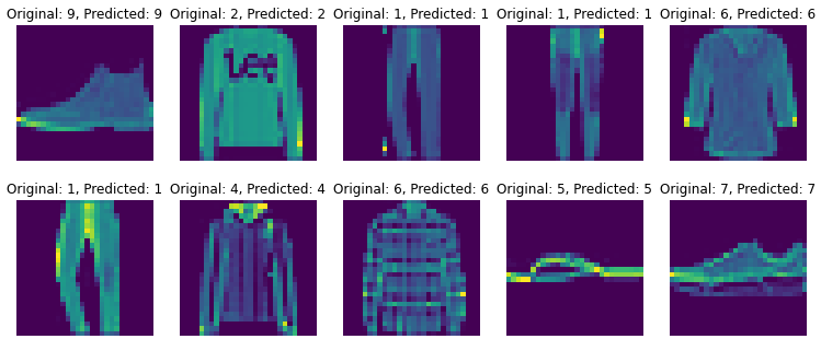
We will now test the model by predicting the first 10 images in the unseen test dataset.
[9 2 1 1 6 1 4 6 5 7]
[9 2 1 1 6 1 4 6 5 7]
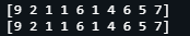
From the above results we can see that our model does a pretty good job in predicting the unseen data.
Let’s visualize the predictions for better insights
Conclusion
In this article, we saw how to classify various clothing items in the Fashion MNIST dataset using an artificial neural network created in the Cainvas Platform.
The Cainvas Platform provides a one stop solution to creating deep learning models which can also be compiled into EDGE device friendly models for using it in your IOT projects. The platform boasts of various other tools and resources to guide you for your next deep learning IOT project.
Implementation of the idea on cAInvas is here!
Credits: Umang Tiwari
Also Read: Next day rain prediction — on cAInvas