Identify sounds that indicate possible danger in the surrounding.

What would your response be if you heard a gunshot or glass break while inside your home? The natural inclination would be to call for help. In most cases, dial the police helpline, a neighbour, a relative, or a friend.
A system to recognize that sounds that indicate possible danger would benefit the neighbourhood. The model underlying the system should be able to recognize the distinct sounds among other background noises. The sounds can then be mapped to the actions to be performed (like calls, notifications, etc) when it is picked up in the surrounding.
In real-time applications, the audio sample is processed run through the model every 0.5 seconds to get predictions. This value is configurable.
In such cases, it is important to remember that false positives are acceptable while false negatives can result in catastrophic consequences.
Implementation of the idea on cAInvas — here!
The dataset
On Kaggle by Chris Gorgolewski
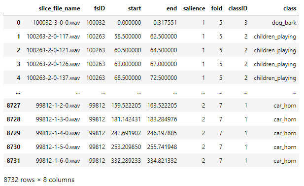
The UrbanSound8K dataset is commonly used for academic research. It contains 8732 labeled sound excerpts of urban sounds from 10 classes — air_conditioner, car_horn, children_playing, dog_bark, drilling, enginge_idling, gun_shot, jackhammer, siren, and street_music.
The classes are drawn from the urban sound taxonomy. Each file is <=4s in duration. The files are pre-sorted into ten folds, each in its own folder named fold1-fold10. In addition to the sound excerpts, a CSV file containing metadata about each excerpt is also provided.
The dataset folder has 10 subfolders — fold 1 to fold 10, each containing audio samples and a CSV file containing the file name of the sliced audio file, its ID, duration of the clip in terms of start and stop time limits, salience (foreground or background), the fold, the target class ID and the class name.
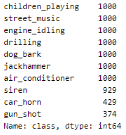
A peek into the distribution of class names —
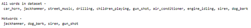
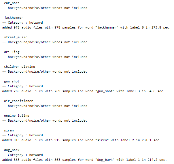
Out of the classes present in the dataset, we pick 4 classes to be our hot words, i.e., classes that define danger.
Defining some important variables for the notebook —
The max_length variable holds the maximum length of the audio clip in the dataset. This value is then multiplied by the sampling rate to be used (desired_sr) to get the desired_samples variable. This is the total number of input variables generated for one audio sample in the dataset. In the case of a sample with a duration of <4s, padding is done.
Defining a few utility functions
Processing the data
The functions below aid in processing the data to be given as input to the model and its output afterward.
The dataset_min and dataset_max are variables that define the minimum and maximum values in the dataset. This is used for normalizing and denormalizing the dataset.
The interpolateAudio function performs 1D linear interpolation on the audio passed using the interp function of the NumPy package.
Handling labels and background samples
Defining functions to handle labeling of samples and inclusion of background noise.
The class_nSamples defines the number of samples to pick from the classes identified as hotwords. This value is divided by the number of words not identified as hotwords to calculate the number of samples to be picked up from each of the other classes to ensure equal distribution among non-hotword samples.
This is the other_nsamples variable and is used only when add_noise is set to True. If add_noise is set to False, classification is done among the n hotword classes.
Creating the dataset
The class names are looped through and if add_noise is False, non-hotwords are not included. In other cases, like hotwords and inclusion of noise, a subset of the data frame with the target column equal to the chosen class name is taken. The audio samples are looped through and in each case, it is loaded using the librosa package.
If the sample is less than 1s long, it is discarded. Other samples are included with/without padding.
Padding is done in those samples whose duration is not a perfect multiple of the max_length variable defines above to achieve the same.
This step is then followed by splitting the audio into samples with a size equal to the desired_samples variable.
The input_labels variable holds the target values as integers. Since the different classes do not have any ordering defined among them, they are one-hot encoded.
For example, if there are 5 classes (0–4) and the target label is 3, the one-hot encoded array will be [0, 0, 0, 1, 0]
Adding noise/silence as background
Background noises include silence and other random noises along with the sounds in the dataset not defined as target classes. We add other_nSamples count of rows for background and silence each.
Silence samples are zero vectors in the shape of the input. Background samples contain random floats in the interval [0.0,1.0).
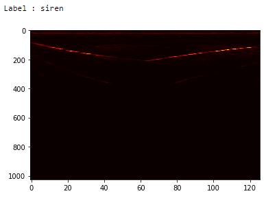
Extracting the STFT (Short-time Fourier transform) features
The sinusoidal frequency and phase content of the audio signals change over time. To retrieve features of the audio clip over long durations, a Fourier-related transform is used on local sections of the signal as it changes over time.
The input dataset now has a shape (3025, 1025, 126).
Train-test split
Shuffling the dataset using a permutation of the indices and splitting it into train and test using a 90–10 ratio.
Playing using inverse-STFT
The processed features are plotted using matplotlib.pyplot package. The istft function of the librosa.core package is used to retrieve the audio file from the STFT features.
Try playing the audio samples in the notebook link above!
The model
The model has a reshape layer that sets the number of channels to 1 in the input given to the model. This is followed by 3 convolutional layers with ReLU activation. The Flatten layer reduces it to 1D which is then passed through 2 Dense layers and a Dropout layer.
The softmax activation function is applied to the output of the Dropout layer. This returns an array of probability values for n classes in the defined dataset, all of which add up to 1.
The Adam optimizer of the tf.keras.optimizers module is used. If there are only two classes in the dataset (two distinct sound classes or a distinct sound and background), the BinaryCrossentropy loss function is used. In all other cases, the CategoricalCrossentropy loss function is used as the labels are one-hot encoded.
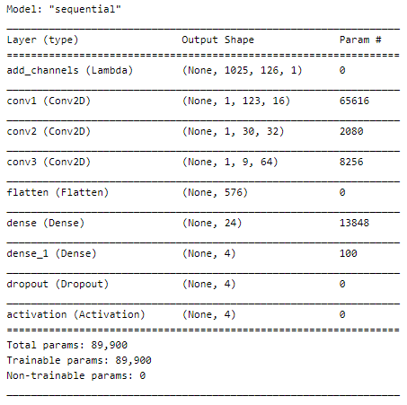
The EarlyStopping callback function of the keras.callbacks module is used to monitor the metrics (default, val_loss) and stop the training if the metric doesn’t improve (increase or decrease based on metric specified) continuously for 20 epochs (patience parameter).
The restore_best_weights parameter is set to true to ensure that the model is loaded with weights corresponding to the checkpoint with the best metric value at the end of the training process.
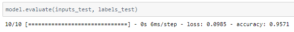
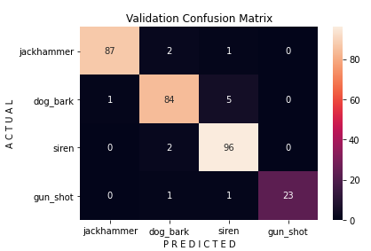
The model is trained with a learning rate of 0.01 and achieves ~95.7% accuracy on the test set.
Prediction
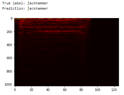
On random sample
Picking a random sample from the test set and performing predictions on it —
On background and silence
Let’s see what the model predicts on silence and background noises —

Confusion matrix
Plotting the confusion matrix —
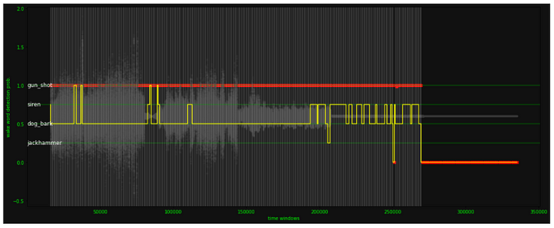
Prediction on longer clips
Multiple audio clips are concatenated one after the other to create a longer clip on which the model is tested.
The audio clip is sampled at regular intervals (Say, 0.02 seconds) and predictions are performed to give continuous outputs. The plot of the predictions helps us understand them better.
Other applications
Common Sounds
Identify the different sounds in your surrounding.
Certain sounds in our surrounding may require a predefined action to be performed on hearing them. Using deep learning to identify them can be used to trigger such actions automatically.
The dataset — On Kaggle by Marc Moreaux
The dataset contains 40 labeled sound excerpts of 5 seconds each from 50 diferent sound classes, making it a total of 2000 audio samples in the dataset.
The dataset was intially proposed by the authors of ESC-50: Dataset for Environmental Sound Classification and further processed by the Kaggle dataset authors mentioned above In addition to the sound excerpts, a CSV file containing metadata about each excerpt is also provided.
deepC
deepC library, compiler, and inference framework are designed to enable and perform deep learning neural networks by focussing on features of small form-factor devices like micro-controllers, eFPGAs, CPUs, and other embedded devices like raspberry-pi, odroid, Arduino, SparkFun Edge, RISC-V, mobile phones, x86 and arm laptops among others.
Head over to the cAInvas platform (link to notebook given earlier) and check out the predictions by the .exe file!
Credits: Ayisha D
Also Read: Surface crack detection — on cAInvas