Predict the quantity of fuel consumed during drives.

The mileage of a vehicle is defined as the average distance traveled on a specified amount of fuel. But distance is not the only factor that affects fuel consumption.
Here, we take into account multiple factors like speed, temperatures inside and outside, AC, and other weather conditions like rain or sun besides distance to predict the consumption of different types of fuels during drives.
Predicting the fuel consumption given distance and other factors vice versa (predicting distance given fuel) can prove useful in planning trips as well as performing real-time predictions during driving.
Implementation of the idea on cAInvas — here!
The dataset
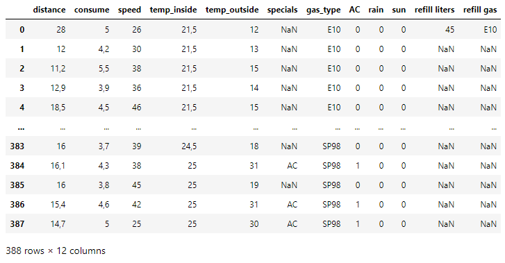
The dataset is a CSV file that was recorded by Andreas on everyday rides by noting factors such as weather (raining or warm), temperatures inside and outside, average speed, etc. in addition to the distance traveled and corresponding fuel consumed per 100 km. The values are recorded for two different types of fuels — E10 and SP98.
(A similar dataset can be used for consumption prediction for any type of fuel)
Data preprocessing
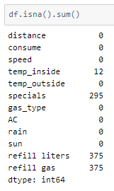
On first look, there are NaN values in the dataset. Checking the dataset for more NaN values —
Filling the NaN values
Mathematical calculations cannot be performed with NaN values. One option would be to drop all rows with NaN values in any one column. The other would be to fill the values with mode, mean or median values of the column depending on its datatype. It is also possible to substitute them with a value that indicates that the value is missing in that row.
The temp_inside column NaN values are filled with mode values corresponding to each category.
The NaN values of the ‘refill liters’ column are substituted with ‘0’ indicating that there was no refilling done.
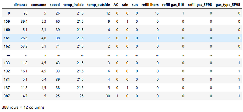
The ‘refill gas’ and ‘gas_type’ columns have categorical values that need to be one-hot encoded. The get_dummies function of the Pandas module is used to get one-hot encoded values for the column values. It is important to note that the ‘refill gas’ column has NaN values.
Setting the dummy_na parameter to True creates a separate column in the list of one hot encoded columns to indicate NaN values. This is later dropped such that rows with NaN value now have 0 in every one hot encoded column.
For example, the ‘refill gas’ column has 3 values — E10, SP98, NaN. The encoding would be as follows — E10→[1,0], SP98→[0,1], NaN →[0,0].
The ‘gas_type’ column is one hot encoded using the same function by setting the drop_first parameter to True resulting in a single column with 0/1 values.
The ‘specials’ column is already one hot encoded into 3 columns — AC, rain, sun. Thus it is dropped.
Checking the datatypes of the columns in the dataset —
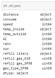
Values in certain columns have ‘,’ in numeric values. In some instances, the decimal point is represented using ‘,’s. These columns end up having the object datatype. Replacing such values with the ‘.’ decimal convention and casting them to float32 data type.
Train-validation-test split
Using a 90–10 ratio to split the data frame into train-validation sets. The train_test_split function of the sklearn.model_selection module is used for this.
The training set has 349 samples and the validation set has 39.
Standardization
The standard deviation of attribute values in the dataset is not the same across all of them. This may result in certain attributes being weighted higher than others. The values across all attributes are scaled to have mean = 0 and standard deviation = 1 with respect to the particular columns.
All the columns in the numeric_columns list need to be standardized except the target column ‘consume’.
The StandardScaler function of the sklearn.preprocessing module is used to implement this concept. The instance is first fit on the training data and then used to transform the train and validation data.
Defining the input and output columns to split into X and y. These are then divided into X and y (input and output) for further processing.
There are 11 input columns and 1 output column.
The model
The model is a simple one with 6 Dense layers, 5 of which have ReLU activation functions and the last one has no activation function that outputs a single value.
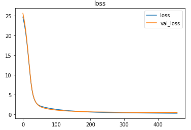
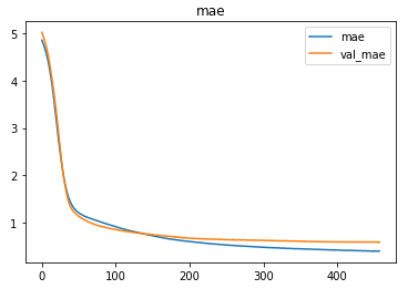
As it is a regression problem, the model is compiled using the mean-squared-error loss function. The Adam optimizer is used and the loss, as well as the mean-absolute-error of the model, is tracked over epochs.
The EarlyStopping callback function of the keras.callbacks module monitors the validation loss and stops the training if it doesn’t decrease for 20 epochs continuously. The restore_best_weights parameter ensures that the model with the least validation loss is restored to the model variable.
The model was trained with a learning rate of 0.00001 and an MSE loss of 0.5256 was achieved on the test set.
The metrics
deepC
deepC library, compiler, and inference framework are designed to enable and perform deep learning neural networks by focussing on features of small form-factor devices like micro-controllers, eFPGAs, CPUs, and other embedded devices like raspberry-pi, odroid, Arduino, SparkFun Edge, RISC-V, mobile phones, x86 and arm laptops among others.
Compiling the model using deepC —
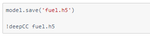
Head over to the cAInvas platform (link to notebook given earlier) and check out the predictions by the .exe file!
Credits: Ayisha D
Also Read: Everyday sound classification for danger identification — on cAInvas